The square root of the probability

Posted on August 19, 2018 by rpflee

Probability amplitude in Layman’s Terms

What I understood is that probability amplitude is the square root of the probability … but the square root of the probability does not mean anything in the physical sense.

Can any please explain the physical significance of the probability amplitude in quantum mechanics?

edited Mar 1 at 16:31
nbro

asked Mar 21 ’13 at 15:36
Deepu

Part of you problem is

“Probability amplitude is the square root of the probability […]”

The amplitude is a complex number whose amplitude is the probability. That is $\psi^* \psi = P$ where the asterisk superscript means the complex conjugate. ${}^{[1]}$ It may seem a little pedantic to make this distinction because so far the “complex phase” of the amplitudes has no effect on the observables at all: we could always rotate any given amplitude onto the positive real line and then “the square root” would be fine.

But we can’t guarantee to be able to rotate more than one amplitude that way at the same time.

More over, there are two ways to combine amplitudes to find probabilities for observation of combined events.

When the final states are distinguishable you add probabilities:

$P_{dis} = P_1 + P_2 = \psi_1^* \psi_1 + \psi_2^* \psi_2$

When the final state are indistinguishable, ${}^{[2]}$ you add amplitudes:

$\Psi_{1,2} = \psi_1 + \psi_2$

and

$P_{ind} = \Psi_{1,2}^*\Psi_{1,2} = \psi_1^*\psi_1 + \psi_1^*\psi_2 + \psi_2^*\psi_1 + \psi_2^* \psi_2$

The terms that mix the amplitudes labeled 1 and 2 are the “interference terms”. The interference terms are why we can’t ignore the complex nature of the amplitudes and they cause many kinds of quantum weirdness.

${}^1$ Here I’m using a notation reminiscent of a Schrödinger-like formulation, but that interpretation is not required. Just accept $\psi$ as a complex number representing the amplitude for some observation.

${}^2$ This is not precise, the states need to be “coherent”, but you don’t want to hear about that today.

edited Mar 21 ’13 at 17:04
answered Mar 21 ’13 at 16:58

dmckee

— Physics Stack Exchange

Number, Time, Money, 3

Posted on August 15, 2018 by rpflee

time ~ change

time interval

~ amount of change

~ quota of change

— Me@2017-09-19 02:48:22 PM

— Me@2018-04-22 06:00:05 PM

神的旨意 2.3

Posted on August 13, 2018 by rpflee

神：我是神，而你只是人。神的心思，凡人不一定能夠理解。所以，作為凡人的你，應該心存謙卑，完全信任你的神，奉行神的旨意。

甲：不合理呀！

如果要殺害無辜，才可上天堂，而不殺害無辜，會被罰落地獄的話，那代表著，你天堂的居民，都是壞人；而你地獄的居民，反而是善人。

那樣，你的所謂「天堂」，根本是我的地獄。而你雖然自封為「神」，卻根本是我的「魔」。

魔：我是魔又如何？我的法力遠高於你。我可以令你求生不得，求死不能。

甲：會有真正善良的神，去保護我。

魔：難保我的法力高過善神。「魔」就不可以是全能的嗎？

甲：如果是全能，你怎會有動機，去虐待凡人呢？既是全能者，又怎會那麼無聊，損人不利己？

另外，如果你法力高強，乃至「全能」，你就不可能是「全惡」的。你必定有善部和惡部。你的善部，就是善神。

魔：為什麼「全能」者不可「全惡」？

…

— Me@2018-08-13 11:54:47 AM

The Jacobian of the inverse of a transformation

Posted on August 9, 2018 by rpflee

The Jacobian of the inverse of a transformation is the inverse of the Jacobian of that transformation

In this post, we would like to illustrate the meaning of

the Jacobian of the inverse of a transformation = the inverse of the Jacobian of that transformation

by proving a special case.

Consider a transformation $\mathscr{T}: \bar{x}^i=\bar{x}^i (x^1,x^2)$ , which is an one-to-one mapping from unbarred $x^i$ ‘s to barred $\bar{x}^i$ coordinates, where $i=1, 2$ .

By definition, the Jacobian matrix J of $\mathscr{T}$ is

$J= \begin{pmatrix} \displaystyle{\frac{\partial \bar{x}^1}{\partial x^1}} & \displaystyle{\frac{\partial \bar{x}^1}{\partial x^2}} \\ \displaystyle{\frac{\partial \bar{x}^2}{\partial x^1}} & \displaystyle{\frac{\partial \bar{x}^2}{\partial x^2}} \end{pmatrix}$

Now we consider the the inverse of the transformation $\mathscr{T}$ :

$\mathscr{T}^{-1}: x^i=x^i(\bar{x}^1,\bar{x}^2)$

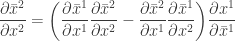
By definition, the Jacobian matrix $\bar{J}$ of this inverse transformation, $\mathscr{T}^{-1}$ , is

$\bar{J}= \begin{pmatrix} \displaystyle{\frac{\partial x^1}{\partial \bar{x}^1}} & \displaystyle{\frac{\partial x^1}{\partial \bar{x}^2}} \\ \displaystyle{\frac{\partial x^2}{\partial \bar{x}^1}} & \displaystyle{\frac{\partial x^2}{\partial \bar{x}^2}} \end{pmatrix}$

On the other hand, the inverse of Jacobian $J$ of the original transformation $\mathscr{T}$ is

$J^{-1}=\displaystyle{\frac{1}{ \begin{vmatrix} \displaystyle{\frac{\partial \bar{x}^1}{\partial x^1}} & \displaystyle{\frac{\partial \bar{x}^1}{\partial x^2}} \\ \displaystyle{\frac{\partial \bar{x}^2}{\partial x^1}} & \displaystyle{\frac{\partial \bar{x}^2}{\partial x^2}} \end{vmatrix} }} \begin{pmatrix} \displaystyle{\frac{\partial \bar{x}^2}{\partial x^2}} & \displaystyle{-\frac{\partial \bar{x}^1}{\partial x^2}} \\ \displaystyle{-\frac{\partial \bar{x}^2}{\partial x^1}} & \displaystyle{\frac{\partial \bar{x}^1}{\partial x^1}} \end{pmatrix}$

If $\bar{J} = J^{-1}$ , their (1, 1)-elementd should be equation:

$\displaystyle{\frac{\partial x^1}{\partial \bar{x}^1}}\stackrel{?}{=}\displaystyle{\frac{1}{\displaystyle{\frac{\partial \bar{x}^1}{\partial x^1}}\displaystyle{\frac{\partial \bar{x}^2}{\partial x^2}}-\displaystyle{\frac{\partial \bar{x}^1}{\partial x^2}}\displaystyle{\frac{\partial \bar{x}^2}{\partial x^1}} }} \bigg( \displaystyle{\frac{\partial \bar{x}^2}{\partial x^2}} \bigg)$

Let’s try to prove that.

Consider equations

$\bar{x}^1 = \bar{x}^1(x^1,x^2)$

$\bar{x}^2 = \bar{x}^2(x^1,x^2)$

Differentiate both sides of each equation with respect to $\bar{x}^1$ , we have:

$A := 1=\displaystyle{\frac{\partial \bar{x}^1}{\partial \bar{x}^1}=\frac{\partial \bar{x}^1}{\partial x^1}\frac{\partial x^1}{\partial \bar{x}^1}+\frac{\partial \bar{x}^1}{\partial x^2}\frac{\partial x^2}{\partial \bar{x}^1}}$

$B := 0 = \displaystyle{\frac{\partial \bar{x}^2}{\partial \bar{x}^1}=\frac{\partial \bar{x}^2}{\partial x^1}\frac{\partial x^1}{\partial \bar{x}^1}+\frac{\partial \bar{x}^2}{\partial x^2}\frac{\partial x^2}{\partial \bar{x}^1}}$

$A \times \displaystyle{\frac{\partial \bar{x}^2}{\partial x^2}}:~~~~~C := \displaystyle{\frac{\partial \bar{x}^2}{\partial x^2}=\frac{\partial \bar{x}^1}{\partial x^1}\frac{\partial x^1}{\partial \bar{x}^1}\frac{\partial \bar{x}^2}{\partial x^2}+\frac{\partial \bar{x}^1}{\partial x^2}\frac{\partial x^2}{\partial \bar{x}^1}\frac{\partial \bar{x}^2}{\partial x^2}}$

$B \times \displaystyle{\frac{\partial \bar{x}^1}{\partial x^2}}:~~~~~D := \displaystyle{0=\frac{\partial \bar{x}^2}{\partial x^1}\frac{\partial x^1}{\partial \bar{x}^1}\frac{\partial \bar{x}^1}{\partial x^2}+\frac{\partial \bar{x}^2}{\partial x^2}\frac{\partial x^2}{\partial \bar{x}^1}\frac{\partial \bar{x}^1}{\partial x^2}}$

$D-C:$

$\displaystyle{ \frac{\partial \bar{x}^2}{\partial x^2}= \bigg( \frac{\partial \bar{x}^1}{\partial x^1}\frac{\partial \bar{x}^2}{\partial x^2} - \frac{\partial \bar{x}^2}{\partial x^1}\frac{\partial \bar{x}^1}{\partial x^2}\bigg) \frac{\partial x^1}{\partial \bar{x}^1}}$ ,

results

$\displaystyle{ \frac{\partial x^1}{\partial \bar{x}^1}}=\frac{\displaystyle{\frac{\partial \bar{x}^2}{\partial x^2}}}{\displaystyle{\frac{\partial \bar{x}^1}{\partial x^1}\frac{\partial \bar{x}^2}{\partial x^2} - \frac{\partial \bar{x}^1}{\partial x^2}\frac{\partial \bar{x}^2}{\partial x^1}}}$

…

— Me@2018-08-09 09:49:51 PM

Problem 14.5a1

Posted on August 7, 2018 by rpflee

Counting states in heterotic $SO(32)$ string theory | A First Course in String Theory

(a) Consider the left NS’ sector. Write the precise mass-squared formula with normal-ordered oscillators and the appropriate normal-ordering constant.

~~~

$\displaystyle{\alpha' M_L^2 = \frac{1}{2} \sum_{n \ne 0} \bar \alpha_{-n}^I \bar \alpha_n^I + \frac{1}{2} \sum_{r \in \mathbf{Z} + \frac{1}{2}}r \lambda_{-r}^A \lambda_r^A}$

What is normal-ordering?

Put all the creation operators on the left.

What for?

p.251 “It is useful to work with normal-ordered operators since they act in a simple manner on the vacuum state. We cannot use operators that do not have a well defined action on the vacuum state.”

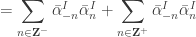
“The vacuum expectation value of a normal ordered product of creation and annihilation operators is zero. This is because, denoting the vacuum state by $|0\rangle$ , the creation and annihilation operators satisfy”

$\displaystyle{\langle 0 | \hat{a}^\dagger = 0 \qquad \textrm{and} \qquad \hat{a} |0\rangle = 0}$

— Wikipedia on Normal order

— This answer is my guess. —

$\displaystyle{\sum_{n \ne 0} \bar \alpha_{-n}^I \bar \alpha_n^I}$

$\displaystyle{= \sum_{n \in \mathbf{Z}^-} \bar \alpha_{-n}^I \bar \alpha_n^I + \sum_{n \in \mathbf{Z}^+} \bar \alpha_{-n}^I \bar \alpha_n^I}$

$\displaystyle{= \sum_{n \in \mathbf{Z}^+} \bar \alpha_{n}^I \bar \alpha_{-n}^I + \sum_{n \in \mathbf{Z}^+} \bar \alpha_{-n}^I \bar \alpha_n^I}$

$\displaystyle{= \sum_{n \in \mathbf{Z}^+} \left[ \bar \alpha_{n}^I \bar \alpha_{-n}^I - \bar \alpha_{-n}^I \bar \alpha_{n}^I + \bar \alpha_{-n}^I \bar \alpha_{n}^I \right] + \sum_{n \in \mathbf{Z}^+} \bar \alpha_{-n}^I \bar \alpha_n^I}$

$\displaystyle{= \sum_{n \in \mathbf{Z}^+} \left[ \bar \alpha_{n}^I, \bar \alpha_{-n}^I \right] + \sum_{n \in \mathbf{Z}^+} \bar \alpha_{-n}^I \bar \alpha_{n}^I + \sum_{n \in \mathbf{Z}^+} \bar \alpha_{-n}^I \bar \alpha_n^I}$

$= \displaystyle{\sum_{n \in \mathbf{Z}^+} n \eta^{II} + 2 \sum_{n \in \mathbf{Z}^+} \bar \alpha_{-n}^I \bar \alpha_{n}^I}$

c.f. p.251:

$\displaystyle{\sum_{n \ne 0} \bar \alpha_{-n}^I \bar \alpha_n^I}$

$\displaystyle{= \sum_{n \in \mathbf{Z}^+} n \eta^{II} + 2 \sum_{n \in \mathbf{Z}^+} \bar \alpha_{-n}^I \bar \alpha_{n}^I}$

$\displaystyle{= \frac{-1}{12} (D - 2) + 2 \sum_{n \in \mathbf{Z}^+} \bar \alpha_{-n}^I \bar \alpha_{n}^I}$

Equation at Problem 14.5:

$\displaystyle{\alpha' M_L^2}$

$\displaystyle{= \frac{1}{2} \sum_{n \ne 0} \bar \alpha_{-n}^I \bar \alpha_n^I + \frac{1}{2} \sum_{r \in \mathbf{Z} + \frac{1}{2}}r \lambda_{-r}^A \lambda_r^A}$

$\displaystyle{= \frac{1}{2} \left[ \frac{-1}{12} (D - 2) + 2 \sum_{n \in \mathbf{Z}^+} \bar \alpha_{-n}^I \bar \alpha_{n}^I \right] + \frac{1}{2} \sum_{r \in \mathbf{Z} + \frac{1}{2}}r \lambda_{-r}^A \lambda_r^A}$

$\displaystyle{= \frac{-1}{24} (D - 2) + \sum_{n \in \mathbf{Z}^+} \bar \alpha_{-n}^I \bar \alpha_{n}^I + \frac{1}{2} \sum_{r \in \mathbf{Z} + \frac{1}{2}}r \lambda_{-r}^A \lambda_r^A}$

$\displaystyle{= \frac{-1}{8} + \sum_{n \in \mathbf{Z}^+} \bar \alpha_{-n}^I \bar \alpha_{n}^I + \frac{1}{2} \sum_{r \in \mathbf{Z} + \frac{1}{2}}r \lambda_{-r}^A \lambda_r^A}$

$D = 10$

$\displaystyle{\sum_{r \in \mathbf{Z} + \frac{1}{2}}r \lambda_{-r}^A \lambda_r^A}$

$\displaystyle{= \sum_{r = - \frac{1}{2}, - \frac{3}{2}, ...} r \lambda_{-r}^A \lambda_r^A + \sum_{r = \frac{1}{2}, \frac{3}{2}, ...} r \lambda_{-r}^A \lambda_r^A}$

$\displaystyle{= \sum_{r = \frac{1}{2}, \frac{3}{2}, ...} (-r) \lambda_{r}^A \lambda_{-r}^A + \sum_{r = \frac{1}{2}, \frac{3}{2}, ...} r \lambda_{-r}^A \lambda_r^A}$

$\displaystyle{= \sum_{r = \frac{1}{2}, \frac{3}{2}, ...} r \left[ (-1) \lambda_{r}^A \lambda_{-r}^A + \lambda_{-r}^A \lambda_r^A \right]}$

$\displaystyle{= \sum_{r = \frac{1}{2}, \frac{3}{2}, ...} r \left[ \lambda_{-r}^A, \lambda_r^A \right]}$

Equation (14.29):

$\displaystyle{\left\{ b_r^I, b_s^J \right\} = \delta_{r+s, 0} \delta^{IJ}}$

$\displaystyle{b_r^I b_s^J = - b_s^I b_r^J + \delta_{r+s, 0} \delta^{IJ}}$

$\displaystyle{\sum_{r \in \mathbf{Z} + \frac{1}{2}}r \lambda_{-r}^A \lambda_r^A}$

$\displaystyle{= \sum_{r = \frac{1}{2}, \frac{3}{2}, ...} r \left[ (-1) \lambda_{r}^A \lambda_{-r}^A + \lambda_{-r}^A \lambda_r^A \right]}$

$\displaystyle{= \sum_{r = \frac{1}{2}, \frac{3}{2}, ...} r \left[ (-1) \left( - \lambda_{-r}^A \lambda_r^A + \delta_{r-r, 0} \delta^{AA} \right) + \lambda_{-r}^A \lambda_r^A \right]}$

$\displaystyle{= \sum_{r = \frac{1}{2}, \frac{3}{2}, ...} r \left[ \lambda_{-r}^A \lambda_r^A + \lambda_{-r}^A \lambda_r^A - 1 \right]}$

$\displaystyle{= \sum_{r = \frac{1}{2}, \frac{3}{2}, ...} r \left[ 2 \lambda_{-r}^A \lambda_r^A - 1 \right]}$

$\displaystyle{\sum_{r \in \mathbf{Z} + \frac{1}{2}}r \lambda_{-r}^A \lambda_r^A}$

$\displaystyle{= - \sum_{r = \frac{1}{2}, \frac{3}{2}, ...} r + \sum_{r = \frac{1}{2}, \frac{3}{2}, ...} r \left[ b_{-r}^A b_r^A + \lambda_{-r}^A \lambda_r^A \right]}$

$\displaystyle{= - \frac{1}{2} \sum_{r = 1, 3, ...} r + \sum_{r = \frac{1}{2}, \frac{3}{2}, ...} r \left[ b_{-r}^A b_r^A + \lambda_{-r}^A \lambda_r^A \right]}$

$\displaystyle{= \left[ - \frac{1}{24} + \sum_{r = \frac{1}{2}, \frac{3}{2}, ...} r \left( b_{-r}^A b_r^A + \lambda_{-r}^A \lambda_r^A \right) \right]}$

— This answer is my guess. —

— Me@2018-08-06 10:23:48 PM

Physics Town

continues

Monthly Archives: August 2018

The square root of the probability

Number, Time, Money, 3

神的旨意 2.3

The Jacobian of the inverse of a transformation

Problem 14.5a1