

.
(autoload 'enable-paredit-mode
  "paredit" "Turn on pseudo-structural editing." t)

(add-hook 'emacs-lisp-mode-hook
      #'enable-paredit-mode)

(add-hook 'eval-expression-minibuffer-setup-hook
      #'enable-paredit-mode)

(add-hook 'ielm-mode-hook
      #'enable-paredit-mode)

(add-hook 'lisp-mode-hook
      #'enable-paredit-mode)

(add-hook 'lisp-interaction-mode-hook
      #'enable-paredit-mode)

(add-hook 'scheme-mode-hook
      #'enable-paredit-mode)


(add-hook 'slime-repl-mode-hook
      (lambda () (paredit-mode +1)))

(defun override-slime-repl-bindings-with-paredit ()
   (define-key slime-repl-mode-map
     (read-kbd-macro paredit-backward-delete-key) nil))

(add-hook 'slime-repl-mode-hook
      'override-slime-repl-bindings-with-paredit)
.

— Me@2022-11-29 10:03:49 PM
.
.
2022.11.29 Tuesday (c) All rights reserved by ACHK


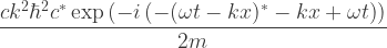


 1 32
QPochhammer[-(-------), x]
Sqrt[x]
------------------------------------
1 32 8
(1 + -------) x QPochhammer[x, x]
Sqrt[x]
                     1        32
    QPochhammer[-(-------), x]
                  Sqrt[x]
------------------------------------
        1    32                    8
(1 + -------)   x QPochhammer[x, x]
     Sqrt[x]


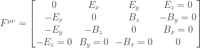
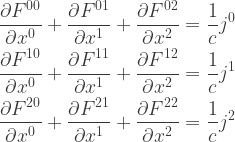
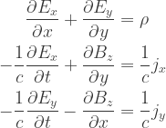
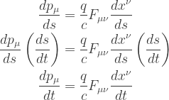
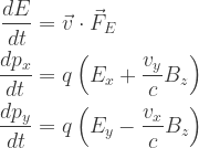
 , examine
  , the Maxwell equations (3.34), and the relativistic form of the force law derived in Problem 3.1.
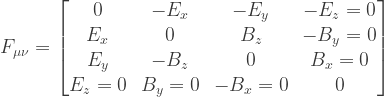


 is obtained from the singularity, you won’t be able to get a good calculation because the integral over the singularity would be singular. Moreover, the space and time are really interchanged inside the black hole (the signs of the components
  and
and  get inverted for
  ) so the exercise is in no way equivalent to a simple 3D volume integral of
 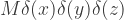 . The Schwarzschild singularity, to pick the "simplest" black hole, is a moment in time, not a place in space. It is the final moment of life for the infalling observers. In a locally (conformally) Minkowski patch near the singularity with some causally Minkowskian coordinates
  and
and 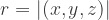 , the Schwarzschild singularity looks like a
  hypersurface, not as
  .
.
You must be logged in to post a comment.