Quantum Methods with Mathematica
.
Assume a wavefunction of the form psi[x, t] == f[t] psi[x] and perform a separation of variables on the wave equation.
Show that f[t] = E^(-I w t) where h w is the separation constant. Try the built-in function DSolve.
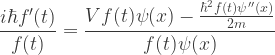
Equate h w to the Energy by evaluating the [expected] value of hamiltonian[V] in the state psi[x, t].
~~~
Remove["Global`*"]


hbar := \[HBar]

H[V_] @ psi_  := -hbar^2/(2m) D[psi,{x,2}] + V psi


psi[x_,t_] := f[t] psi[x]

I hbar D [psi[x,t],t] == H[V] @ psi[x, t]

I hbar D [psi[x,t],t] / psi[x,t] == H[V] @ psi[x,t] / psi[x,t]

E1 := I hbar D [psi[x,t],t] / psi[x,t] == H[V] @ psi[x,t] / psi[x,t]

Simplify[E1]

E2 := - 1/2 hbar hbar (D[D[psi[x],x],x]/(m psi[x])) == hbar omega

DSolve[E2, psi[x], x]


E3 := 1/2 hbar 2 i D[f[t],t] / f[t] == hbar omega

DSolve[E3, f[t], t]


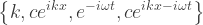
k

psi[x_] := c E^(I k x)

psi[x]

f[t_] := E^(-I omega t)

f[t]

psi[x_,t_] := f[t] psi[x]

psi[x,t]
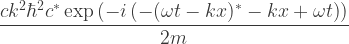
E4 := Conjugate[psi[x,t]] H[0] @ psi[x,t]

E4

E5 := Simplify[E4]

E5

k := Sqrt[2 m omega / hbar]

Refine[E5, {Element[{c, omega, m, t, hbar, k, x}, Reals]}]

E6 := Conjugate[psi[x,t]] psi[x,t]

Simplify[E6]


.

.
— Me@2022-11-26 07:17:29 PM
.
.
2022.11.28 Monday (c) All rights reserved by ACHK


 ,
,  and
and  :
:

 slides off a horizontal cylinder of radius
  in a uniform gravitational field with acceleration
  . If the particle starts close to the top of the cylinder with zero initial speed, with what angular velocity does it leave the cylinder?


 equals
  ,
,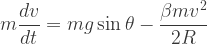
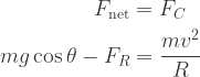 ,
, is the normal reaction force.
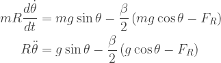
 is still not known. So we keep using the original equation:
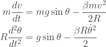


 .
.


 1 32
QPochhammer[-(-------), x]
Sqrt[x]
------------------------------------
1 32 8
(1 + -------) x QPochhammer[x, x]
Sqrt[x]
                     1        32
    QPochhammer[-(-------), x]
                  Sqrt[x]
------------------------------------
        1    32                    8
(1 + -------)   x QPochhammer[x, x]
     Sqrt[x]


You must be logged in to post a comment.