Relationship with other interpretations
The only group of interpretations of quantum mechanics with which RQM is almost completely incompatible is that of hidden variables theories. RQM shares some deep similarities with other views, but differs from them all to the extent to which the other interpretations do not accord with the “relational world” put forward by RQM.
Copenhagen interpretation
RQM is, in essence, quite similar to the Copenhagen interpretation, but with an important difference. In the Copenhagen interpretation, the macroscopic world is assumed to be intrinsically classical in nature, and wave function collapse occurs when a quantum system interacts with macroscopic apparatus. In RQM, any interaction, be it micro or macroscopic, causes the linearity of Schrödinger evolution to break down. RQM could recover a Copenhagen-like view of the world by assigning a privileged status (not dissimilar to a preferred frame in relativity) to the classical world. However, by doing this one would lose sight of the key features that RQM brings to our view of the quantum world.
Hidden variables theories
Bohm’s interpretation of QM does not sit well with RQM. One of the explicit hypotheses in the construction of RQM is that quantum mechanics is a complete theory, that is it provides a full account of the world. Moreover, the Bohmian view seems to imply an underlying, “absolute” set of states of all systems, which is also ruled out as a consequence of RQM.
We find a similar incompatibility between RQM and suggestions such as that of Penrose, which postulate that some processes (in Penrose’s case, gravitational effects) violate the linear evolution of the Schrödinger equation for the system.
Relative-state formulation
The many-worlds family of interpretations (MWI) shares an important feature with RQM, that is, the relational nature of all value assignments (that is, properties). Everett, however, maintains that the universal wavefunction gives a complete description of the entire universe, while Rovelli argues that this is problematic, both because this description is not tied to a specific observer (and hence is “meaningless” in RQM), and because RQM maintains that there is no single, absolute description of the universe as a whole, but rather a net of inter-related partial descriptions.
Consistent histories approach
In the consistent histories approach to QM, instead of assigning probabilities to single values for a given system, the emphasis is given to sequences of values, in such a way as to exclude (as physically impossible) all value assignments which result in inconsistent probabilities being attributed to observed states of the system. This is done by means of ascribing values to “frameworks”, and all values are hence framework-dependent.
RQM accords perfectly well with this view. However, the consistent histories approach does not give a full description of the physical meaning of framework-dependent value (that is it does not account for how there can be “facts” if the value of any property depends on the framework chosen). By incorporating the relational view into this approach, the problem is solved: RQM provides the means by which the observer-independent, framework-dependent probabilities of various histories are reconciled with observer-dependent descriptions of the world.
— Wikipedia on Relational quantum mechanics
.
.
2020.09.27 Sunday ACHK


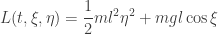


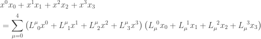
 &= (t; \theta(t); D\theta(t)) \\ \end{aligned}}](https://s0.wp.com/latex.php?latex=%5Cdisplaystyle%7B+%5Cbegin%7Baligned%7D+++%5CGamma%5Bq%5D%28t%29+%26%3D+%28t%3B+%5Ctheta%28t%29%3B+D%5Ctheta%28t%29%29+%5C%5C+++%5Cend%7Baligned%7D%7D&bg=ffffff&fg=333333&s=0&c=20201002)
![\displaystyle{ \begin{aligned} \partial_1 L \circ \Gamma[q] (t) &= - m g l \sin \theta \\ \partial_2 L \circ \Gamma[q] (t) &= m l^2 D \theta \\ \end{aligned}}](https://s0.wp.com/latex.php?latex=%5Cdisplaystyle%7B+%5Cbegin%7Baligned%7D+++%5Cpartial_1+L+%5Ccirc+%5CGamma%5Bq%5D+%28t%29+%26%3D+-+m+g+l+%5Csin+%5Ctheta+%5C%5C++%5Cpartial_2+L+%5Ccirc+%5CGamma%5Bq%5D+%28t%29+%26%3D+m+l%5E2+D+%5Ctheta++%5C%5C++%5Cend%7Baligned%7D%7D&bg=ffffff&fg=333333&s=0&c=20201002)
![\displaystyle{ \begin{aligned} D ( \partial_2 L \circ \Gamma[q]) - (\partial_1 L \circ \Gamma[q]) &= 0 \\ D ( m l^2 D \theta ) - ( - m g l \sin \theta ) &= 0 \\ D^2 \theta + \frac{g}{l} \sin \theta &= 0 \\ \end{aligned}}](https://s0.wp.com/latex.php?latex=%5Cdisplaystyle%7B+%5Cbegin%7Baligned%7D+++D+%28+%5Cpartial_2+L+%5Ccirc+%5CGamma%5Bq%5D%29+-+%28%5Cpartial_1+L+%5Ccirc+%5CGamma%5Bq%5D%29+%26%3D+0+%5C%5C+++D+%28++m+l%5E2+D+%5Ctheta++%29+-+%28+-+m+g+l+%5Csin+%5Ctheta+%29+%26%3D+0+%5C%5C+++D%5E2+%5Ctheta+%2B+%5Cfrac%7Bg%7D%7Bl%7D+%5Csin+%5Ctheta+%26%3D+0+%5C%5C+++%5Cend%7Baligned%7D%7D&bg=ffffff&fg=333333&s=0&c=20201002)


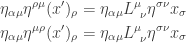
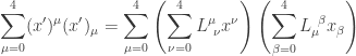
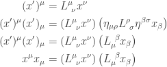
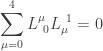
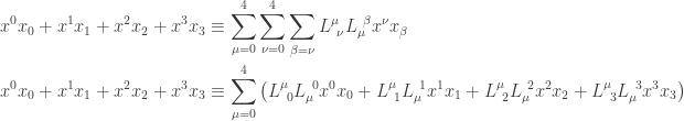
![\displaystyle{\eta_{\alpha \mu} L^\mu_{~\nu} \eta^{\sigma \nu} = \left[L^{-1}\right]^\sigma_{~\alpha}}](https://s0.wp.com/latex.php?latex=%5Cdisplaystyle%7B%5Ceta_%7B%5Calpha+%5Cmu%7D+L%5E%5Cmu_%7B%7E%5Cnu%7D+%5Ceta%5E%7B%5Csigma+%5Cnu%7D+%3D+%5Cleft%5BL%5E%7B-1%7D%5Cright%5D%5E%5Csigma_%7B%7E%5Calpha%7D%7D&bg=ffffff&fg=333333&s=0&c=20201002) .
.
 , the question becomes
![\displaystyle{ \eta_{\mu \rho} L^\rho_{~\sigma} \eta^{\nu \sigma} = \left[L^{-1}\right]^\nu_{~\mu}}](https://s0.wp.com/latex.php?latex=%5Cdisplaystyle%7B+%5Ceta_%7B%5Cmu+%5Crho%7D+L%5E%5Crho_%7B%7E%5Csigma%7D+%5Ceta%5E%7B%5Cnu+%5Csigma%7D+%3D+%5Cleft%5BL%5E%7B-1%7D%5Cright%5D%5E%5Cnu_%7B%7E%5Cmu%7D%7D&bg=ffffff&fg=333333&s=0&c=20201002) .
.
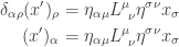
 as
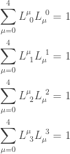
as  . Then the question is simplified to
![\displaystyle{ L^{~\nu}_{\mu} = \left[L^{-1}\right]^\nu_{~\mu}}](https://s0.wp.com/latex.php?latex=%5Cdisplaystyle%7B+L%5E%7B%7E%5Cnu%7D_%7B%5Cmu%7D+%3D+%5Cleft%5BL%5E%7B-1%7D%5Cright%5D%5E%5Cnu_%7B%7E%5Cmu%7D%7D&bg=ffffff&fg=333333&s=0&c=20201002) .
.


 . So the left hand side can be replaced by
  .
.

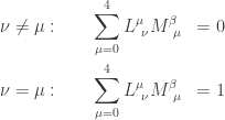
 , such as
  and
and  ,
,
 .
.
 . So
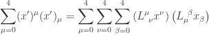
. So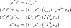

You must be logged in to post a comment.