
You think you know when you learn, are more sure when you can write, even more when you can teach, but certain when you can program.
— Alan Perlis
.
.
2025.10.13 Monday ACHK

You think you know when you learn, are more sure when you can write, even more when you can teach, but certain when you can program.
— Alan Perlis
.
.
2025.10.13 Monday ACHK
Understanding the Euler-Lagrange Operator
.
Let 


Demonstrate the following properties:
a.
…
d.
~~~
Eq. (1.167):
Eq. (1.174):
.
— Me@2025-05-30 03:40:41 PM
.
Prove that
 : time,
 : generalized coordinate (e.g., position),
 : velocity,
 for simplicity.
 : A scalar function of the local tuple, such as
  , akin to a Lagrangian in mechanics.
 : A function that maps one local tuple to another. For example,
  , where
  and
and  transform the coordinate and velocity.
 : This is evaluated at the transformed tuple:
  .
. : For a function
  , it’s defined as:
![\displaystyle{ E[G] = \frac{\partial G}{\partial q} - D_t \left( \frac{\partial G}{\partial v} \right) }](https://s0.wp.com/latex.php?latex=%5Cdisplaystyle%7B+E%5BG%5D+%3D+%5Cfrac%7B%5Cpartial+G%7D%7B%5Cpartial+q%7D+-+D_t+%5Cleft%28+%5Cfrac%7B%5Cpartial+G%7D%7B%5Cpartial+v%7D+%5Cright%29+%7D&bg=ffffff&fg=333333&s=1&c=20201002)
 : This accounts for how a function changes over time, considering all variables. For
  :
:
 is acceleration.
 : The derivative of with respect to its spatial arguments, typically
  .
.…
— Me@2025-05-31 01:32:05 PM
.
.
2025.06.03 Tuesday (c) All rights reserved by ACHK
Structure and Interpretation of Classical Mechanics
.
…
2. On the other hand, the path function ![\bar f[q]](https://s0.wp.com/latex.php?latex=%5Cbar+f%5Bq%5D&bg=ffffff&fg=333333&s=1&c=20201002)
![\bar \Gamma (\bar f) \circ \Gamma [q]](https://s0.wp.com/latex.php?latex=%5Cbar+%5CGamma+%28%5Cbar+f%29+%5Ccirc+%5CGamma+%5Bq%5D&bg=ffffff&fg=333333&s=1&c=20201002)
…
4. Write programs to illustrate the behavior.
~~~
(pp Gamma)

(define ((f-bar q) t)
  (f ((Gamma q) t)))

(define ((Gamma-bar h-bar) local)
  ((h-bar (osculating-path local)) (time local)))

(define (q t)
  (sin t))

(define (f-bar q)
  (D q))

(define p
  (literal-function 'q))

(show-expression
 ((f-bar p) 't))
(show-expression
 ((osculating-path ((Gamma p) 't_0)) 't))
(show-expression
 ((Gamma-bar f-bar) ((Gamma p) 't)))
(define ((GammaBar-fBar-o-Gamma f-bar) q)
  (compose (Gamma-bar f-bar) (Gamma q)))

(show-expression
 (((GammaBar-fBar-o-Gamma f-bar) p) 't))
Two paths that have the same local description up to the
-th derivative are said to osculate with order-
(define (g-bar q)
  ((expt D 3) q))

(show-expression
 ((Gamma p) 't))
(show-expression
 ((g-bar p) 't))
(show-expression
 ((osculating-path ((Gamma p) 't_0)) 't))
(show-expression
 (((GammaBar-fBar-o-Gamma g-bar) p) 't))
— Me@2024-10-16 10:34:35 AM
.
.
2025.02.16 Sunday (c) All rights reserved by ACHK
Structure and Interpretation of Classical Mechanics
.
…
2. On the other hand, the path function
3. Give examples where they are the same and where they are not the same.
…
~~~
…
In other words, path 


.
The second case is when the path function ![\bar f [q]](https://s0.wp.com/latex.php?latex=%5Cbar+f+%5Bq%5D&bg=ffffff&fg=333333&s=1&c=20201002)


Assume that the path is 
and ![\displaystyle{\bar f [q] = Dq}](https://s0.wp.com/latex.php?latex=%5Cdisplaystyle%7B%5Cbar+f+%5Bq%5D+%3D+Dq%7D&bg=ffffff&fg=333333&s=1&c=20201002)
Then  = \cos (t_0)}](https://s0.wp.com/latex.php?latex=%5Cdisplaystyle%7B%5Cbar+f+%5Bq%5D%28t+%3D+t_0%29+%3D+%5Ccos+%28t_0%29%7D&bg=ffffff&fg=333333&s=1&c=20201002)
.
== a taylor series with finite length
.
However, if a path function 

![\displaystyle{\bar g [q] = D^3q}](https://s0.wp.com/latex.php?latex=%5Cdisplaystyle%7B%5Cbar+g+%5Bq%5D+%3D+D%5E3q%7D&bg=ffffff&fg=333333&s=1&c=20201002)
then  = - \cos (t_0)}](https://s0.wp.com/latex.php?latex=%5Cdisplaystyle%7B%5Cbar+g+%5Bq%5D%28t+%3D+t_0%29+%3D+-+%5Ccos+%28t_0%29%7D&bg=ffffff&fg=333333&s=1&c=20201002)
— Me@2025-01-12 06:43:55 AM
.
.
2025.01.12 Sunday (c) All rights reserved by ACHK
Scheme Mechanics Installation for GNU/Linux | scmutils, 4
.
1. Folks, the scmutils library is fantastic and it’s available in Ubuntu 24.04. You can install it very easily with this command:
sudo apt-get install scmutils
2. Then, you just run it with this command:
mit-scheme --band mechanics.com

.
Now, let me tell you, there’s no syntax highlighting. Not great! And more importantly, there’s no direct way to save your code. So, what do you do? You use the Emacs editor. It’s the best!
Now, this assumes you know
Emacs. If you don’t, it’s a tremendous editor.
3. Open Emacs’ initialization file. It’s located right here:
~/.emacs
4. Add this beautiful code to the file:
(defun mechanics ()
  (interactive)
  (run-scheme
   "mit-scheme --band mechanics.com"))
(setq sicm-file "~/Documents/tt.scm")

(fset 'set-working-file
      (lambda (&optional arg)
        (interactive "p")
        (funcall (lambda ()
                   (insert
                    (concat "(define sicm-file \""
                            sicm-file
                            "\")\n"))))))

(fset 'load-scm
      (lambda (&optional arg)
        (interactive "p")
        (funcall (lambda ()
                   (insert "(load sicm-file)")))))

(defun mechan ()
  (interactive)
  (split-window-below)
  (windmove-down)
  (mechanics)
  (set-working-file)
  (comint-send-input)
  (windmove-up)
  (find-file sicm-file)
  (end-of-buffer)
  (windmove-down)
  (cond ((file-exists-p sicm-file)
         (interactive)
         (load-scm)
         (comint-send-input)))
  (windmove-up))

(defun sicm-exec-line ()
  (interactive)
  (save-buffer)
  (windmove-down)
  (comint-send-input)
  (windmove-up))

(defun sicm-exec-file ()
  (interactive)
  (save-buffer)
  (windmove-down)
  (load-scm)
  (comint-send-input)
  (windmove-up))

(global-set-key (kbd "C-x C-e") 'sicm-exec-line)

(global-set-key (kbd "C-x C-a") 'sicm-exec-file)
5. Close Emacs and then re-open it, folks.
6. Type the command
M-x mechan
Now, listen, when I say M-x, I mean you press the Alt key and x together. Then, just type mechan. It’s easy, believe me!
7. You’ll see the Emacs editor split into two windows, one on top and one on the bottom.
The lower window is the Scheme environment. You can type a line of code and then press Enter to execute it. So simple!

The upper window is the editor. Type multiple lines of code and then hit
C-x C-e
to execute it.
That means pressing Ctrl and x together, then Ctrl and e together. Easy stuff!
8. When you save the current file, your Scheme code will be saved to this location:
~/Documents/tt.scm
If you need to back up your code, just back up this file. It’s that simple, folks!
— Me@2020-03-10 10:59:45 PM
.
.
2024.12.01 Sunday (c) All rights reserved by ACHK
Structure and Interpretation of Classical Mechanics
.
1. The local-tuple function 

![\bar f[q] = f \circ \Gamma [q]](https://s0.wp.com/latex.php?latex=%5Cbar+f%5Bq%5D+%3D+f+%5Ccirc+%5CGamma+%5Bq%5D&bg=ffffff&fg=333333&s=1&c=20201002)
2. On the other hand, the path function
…
~~~
1. …
To summarize:
In theory where a series can have infinite terms, functions 
In practice where a series can have only finite terms, they are still identical because their inputs are the same exact local tuples.
2. However, for 

![\Gamma[q]](https://s0.wp.com/latex.php?latex=%5CGamma%5Bq%5D&bg=ffffff&fg=333333&s=1&c=20201002)
(define ((GammaBar-fBar-o-Gamma f-bar) q)
  (compose (Gamma-bar f-bar) (Gamma q)))
Then it would use the function osculating-path to generate the path.
(define ((Gamma-bar f-bar) local)
  ((f-bar (osculating-path local)) (time local)))
In other words, the path being used is the osculating path

instead of the original path
The first case is when

where

In other words, path
The second case is when the path function
…
— Me@2024-10-16 10:34:35 AM
.
.
2024.11.17 Sunday (c) All rights reserved by ACHK
Structure and Interpretation of Classical Mechanics
.
1. The local-tuple function
2. …
~~~
1. Equation
is the definition of
is the definition of
is just true by definition.
In practice, their initial inputs are both the same local tuple

which has only a finite number of components. The path
So the function
.
In other words, since for the functions 

Conceptually,
(define (f local)
  (g local))

(define ((Gamma-bar f-bar) local)
  ((f-bar (osculating-path local)) (time local)))

(define ((f-bar q) t)
  (f ((Gamma q) t))

;; (((f-bar q) 't)
;; == f((Gamma q) 't)
;; == f('t, (v 't), (a 't),...)
— Me@2024-10-16 10:34:35 AM
.
.
2024.11.04 Monday (c) All rights reserved by ACHK
Structure and Interpretation of Classical Mechanics
.
In classical mechanics, there are scenarios where the path function cannot be reconstructed from a finite number of local tuples, such as time 


Consider a system exhibiting chaotic behavior, such as the double pendulum. In this system, the motion is highly sensitive to initial conditions, meaning that even small changes in the initial state can lead to vastly different trajectories over time.
Path Reconstruction Failure: In chaotic systems, the trajectory can diverge significantly from nearby trajectories. Thus, even if you have the position 
In summary, chaotic systems like the double pendulum illustrate how the path function cannot be reconstructed from a finite number of local tuples due to their sensitive dependence on initial conditions and the complexity of their dynamics. This highlights the limitations of local information in capturing the full behavior of certain mechanical systems.
— AI
.
.
2024.10.18 Friday (c) All rights reserved by ACHK
Structure and Interpretation of Classical Mechanics
.
Use the procedure Gamma-bar to construct a procedure that transforms velocities given a coordinate transformation. Apply this procedure to the procedure p->r to deduce (again) equation (1.65).
~~~
(define ((Gamma-bar f-bar) path-q-local-tuple)
  (let* ((tqva path-q-local-tuple)
         (t (time tqva))
         (O-tqva (osculating-path tqva)))
    ((f-bar O-tqva) t)))

(define (F->C F)
  (define (f-bar q-prime)
    (define q
      (compose F (Gamma q-prime)))
    (Gamma q))
  (Gamma-bar f-bar))

(define (F->v F)
  (compose velocity (F->C F)))

(show-expression
 ((F->v p->r)
  (->local 't
           (up 'r 'theta)
           (up 'rdot 'thetadot))))
— Me@2024-09-13 07:17:24 PM
.
.
2024.09.13 Friday (c) All rights reserved by ACHK
Structure and Interpretation of Classical Mechanics
.
…
3. The key point is that since 


Note that it is not the definition of ![\bar f[q']](https://s0.wp.com/latex.php?latex=%5Cbar+f%5Bq%27%5D&bg=ffffff&fg=333333&s=1&c=20201002)
(define (F->C F)
  (define (f-bar q-prime)
    (define q
      (compose F (Gamma q-prime)))
    (Gamma q))
  (Gamma-bar f-bar))
4. However, in the original definition,
(define ((F->C F) local)
  (->local (time local)
           (F local)
           (+ (((partial 0) F) local)
              (* (((partial 1) F) local)
                 (velocity local)))))
there are some partial differentiation operators. Where are they in the new definition?
Those partial differentiation operators are within the definition of the function osculating-path.
(define ((Gamma-bar f-bar) path-q-local-tuple)
  (let* ((tqva path-q-local-tuple)
         (t (time tqva))
         (O-tqva (osculating-path tqva)))
    ((f-bar O-tqva) t)))
— Me@2024-06-13 03:47:47 PM
.
.
2024.08.28 Wednesday (c) All rights reserved by ACHK
Structure and Interpretation of Classical Mechanics
.
(define ((F->C F) local)
  (->local (time local)
           (F local)
           (+ (((partial 0) F) local)
              (* (((partial 1) F) local)
                 (velocity local)))))
The goal of this post is to explain why the code above can be replaced by the following code:
(define (F->C F)
  (define (f-bar q-prime)
    (define q
      (compose F (Gamma q-prime)))
    (Gamma q))
  (Gamma-bar f-bar))
.
While the input of 


.
Let us define
The difference between 

The explicit form of
(define ((Gamma-bar f-bar) path-q-local-tuple)
  (let* ((tqva path-q-local-tuple)
         (t (time tqva))
         (O-tqva (osculating-path tqva)))
    ((f-bar O-tqva) t)))
Note that
.
What is
Equation (1.68):
While 
Equation (1.74):
Note that:
1. The input of 

2. The symbol
…
— Me@2024-08-05 10:09:25 PM
.
.
2024.08.05 Monday (c) All rights reserved by ACHK
Structure and Interpretation of Classical Mechanics
.
Let 
So, to get a value of 
(define ((Gamma-bar f-bar) path-q-local-tuple)
  (let* ((tqva path-q-local-tuple)
         (t (time tqva))
         (O-tqva (osculating-path tqva)))
    ((f-bar O-tqva) t)))
.
The procedure
osculating-pathtakes a number of local components and returns a path with these components; it is implemented as a power series.
In scmutils, you can use the pp function to get the definition of a function. For example, the code
(pp osculating-path)
results
(define ((osculating-path state0) t)
  (let ((t0 (time state0))
        (q0 (coordinate state0))
        (k (vector-length state0)))
    (let ((dt (- t t0)))
      (let loop ((n 2) (sum q0) (dt^n/n! dt))
        (if (fix:= n k)
            sum
            (loop (+ n 1)
                  (+ sum
                     (* (vector-ref state0 n)
                        dt^n/n!))
                  (/ (* dt^n/n! dt) n)))))))
.
Note that for the function in the program, 


.
(define (F->C F)
  (define (f-bar q-prime)
    (define q
      (compose F (Gamma q-prime)))
    (Gamma q))
  (Gamma-bar f-bar))

(show-expression
 ((F->C p->r)
  (->local 't
           (up 'r 'theta)
           (up 'rdot 'thetadot))))
— Me@2023-12-19 08:16:40 PM
.
.
2024.06.15 Saturday (c) All rights reserved by ACHK
Structure and Interpretation of Classical Mechanics
.
Given a function
of a local tuple, a corresponding path-dependent function
is
.
So while the input of
.
Given
we can reconstitute
1. The goal is to use
2. The argument of
3. Assume that we have the value of the initial position of the path, 

Note that while 
Knowing the value of
— Me@2023-12-19 08:16:40 PM
.
.
2024.01.29 Monday (c) All rights reserved by ACHK
Series can also be formed by processes such as exponentiation of an

operator or a square matrix.  For example, if f is any function of one

argument, and if x and dx are numerical expressions, then this

expression denotes the Taylor expansion of f around x.
(((exp (* dx D)) f) x)

= (+ (f x) (* dx ((D f) x)) (* 1/2 (expt dx 2) (((expt D 2) f) x)) ...)
— refman
.
(((exp (* 'dx D)) (literal-function 'f)) 'x)
(show-expression
 (series:print (((exp (* 'dx D))
                 (literal-function 'f)) 'x)))
(f x)
(* dx ((D f) x))
(* 1/2 (expt dx 2) (((expt D 2) f) x))
(* 1/6 (expt dx 3) (((expt D 3) f) x))
(* 1/24 (expt dx 4) (((expt D 4) f) x))
(* 1/120 (expt dx 5) (((expt D 5) f) x))
(* 1/720 (expt dx 6) (((expt D 6) f) x))
(* 1/5040 (expt dx 7) (((expt D 7) f) x))
(* 1/40320 (expt dx 8) (((expt D 8) f) x))
(* 1/362880 (expt dx 9) (((expt D 9) f) x))
(* 1/3628800 (expt dx 10) (((expt D 10) f) x))
(* 1/39916800 (expt dx 11) (((expt D 11) f) x))
(* 1/479001600 (expt dx 12) (((expt D 12) f) x))
(* 1/6227020800 (expt dx 13) (((expt D 13) f) x))
(* 1/87178291200 (expt dx 14) (((expt D 14) f) x))
;Aborting!: maximum recursion depth exceeded
— Me@2023-12-20 11:30:50 AM
.
.
2023.12.20 Wednesday (c) All rights reserved by ACHK
1. …
2. However, there are more general symmetries that no coordinate system can fully express. For example, motion in a central potential is spherically symmetric … , but the expression of the Lagrangian for the system in spherical coordinates exhibits symmetry around only one axis.
3. …
4. A continuous symmetry is a parametric family of symmetries. Noether proved that for any continuous symmetry there is a conserved quantity.
— Structure and Interpretation of Classical Mechanics
.
.
2023.10.23 Monday ACHK
Structure and Interpretation of Classical Mechanics
.
…
What symmetry(ies) can you have?
Find coordinates that express the symmetry.
What is conserved?
Give [the] analytic expression(s) for the conserved quantity(ies).
~~~
[guess]
…
(define ((F->C F) local)
  (->local (time local)
           (F local)
           (+ (((partial 0) F) local)
              (* (((partial 1) F) local)
                 (velocity local)))))

(define (L-driven m R qs U)
  (compose
   (L-rect m R qs U)
   (F->C (sf->rf qs))))

(let* ((U (U-gravity 'g 'm))
       (xs (lambda (t) 0))
       (ys (lambda (t) 0))
       (zs (literal-function 'z_s))
       (qs (up xs ys zs))
       (L (L-driven 'm 'R qs U))
       (q (up (literal-function 'r)
              (literal-function 'theta)
              (literal-function 'phi)
              (literal-function 'lambda))))
  (show-expression
   ((compose L (Gamma q)) 't)))
(+ (* 1/2 m (expt (r t) 2)
            (expt (sin (theta t)) 2)
            (expt ((D phi) t) 2))
   (* -1 m ((D z_s) t)
           (r t)
           (sin (theta t))
           ((D theta) t))
   (* 1/2 m (expt (r t) 2)
            (expt ((D theta) t) 2))
   (* -1 g m (cos (theta t)) (r t))
   (* m ((D r) t)
        ((D z_s) t)
        (cos (theta t)))
   (* (expt R 2) (lambda t))
   (* -1 g m (z_s t))
   (* 1/2 m (expt ((D r) t) 2))
   (* 1/2 m (expt ((D z_s) t) 2))
   (* -1 (lambda t) (expt (r t) 2)))
(let* ((U (U-gravity 'g 'm))
       (xs (lambda (t) 0))
       (ys (lambda (t) 0))
       (zs (literal-function 'z_s))
       (qs (up xs ys zs))
       (L (L-driven 'm 'R qs U))
       (q (up (literal-function 'r)
              (literal-function 'theta)
              (literal-function 'phi)
              (literal-function 'lambda))))
  (show-expression
   (((Lagrange-equations L) q) 't)))
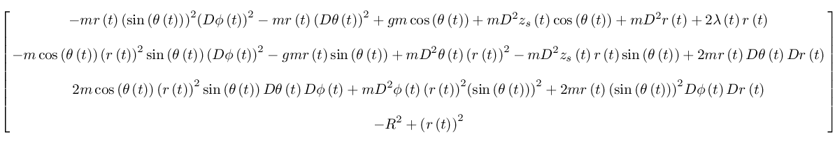
(let* ((U (U-gravity 'g 'm))
       (xs (lambda (t) 0))
       (ys (lambda (t) 0))
       (zs (literal-function 'z_s))
       (qs (up xs ys zs))
       (L (L-driven 'm 'R qs U))
       (q (up (literal-function 'r)
              (literal-function 'theta)
              (literal-function 'phi)
              (literal-function 'lambda))))
  (show-expression
   ((compose (Lagrangian->energy L) (Gamma q)) 't)))

(let* ((U (U-gravity 'g 'm))
       (xs (lambda (t) 0))
       (ys (lambda (t) 0))
       (zs (literal-function 'z_s))
       (qs (up xs ys zs))
       (L (L-driven 'm 'R qs U))
       (q (up (literal-function 'r)
              (literal-function 'theta)
              (literal-function 'phi)
              (literal-function 'lambda))))
  (show-expression
   ((compose ((partial 1) L) (Gamma q)) 't)))

The
component of the force is zero because
(let* ((U (U-gravity 'g 'm))
       (xs (lambda (t) 0))
       (ys (lambda (t) 0))
       (zs (literal-function 'z_s))
       (qs (up xs ys zs))
       (L (L-driven 'm 'R qs U))
       (q (up (literal-function 'r)
              (literal-function 'theta)
              (literal-function 'phi)
              (literal-function 'lambda))))
  (show-expression
   ((compose ((partial 2) L) (Gamma q)) 't)))

[guess]
— Me@2023-08-20 05:02:09 PM
.
.
2023.09.15 Friday (c) All rights reserved by ACHK
This equation is complete. It has meaning independent of the context and there is nothing left to the imagination. The earlier equations require the reader to fill in lots of detail that is implicit in the context. They do not have a clear meaning independent of the context.
— Functional Differential Geometry
.
.
2023.09.05 Tuesday ACHK
Structure and Interpretation of Classical Mechanics
.
A spherical pendulum is a massive bob, subject to uniform gravity, that may swing in three dimensions, but remains at a given distance from the pivot.
Formulate a Lagrangian for a spherical pendulum, driven by vertical motion of the pivot.
…
~~~
How come [the equations]?
Maybe just using the above equation but set the 
to add a something in order to realize the moving center.
— Me@2006
.
[guess]
(define (KE-particle m v)
  (* 1/2 m (square v)))

(define ((extract-particle pieces) local i)
  (let* ((indices (apply up
                         (iota pieces
                               (* i pieces))))
         (extract (lambda (tuple)
                    (vector-map
                     (lambda (i) (ref tuple i))
                     indices))))
    (up (time local)
        (extract (coordinate local))
        (extract (velocity local)))))

(define (U-constraint R qs q lambd)
  (* lambd
     (- (square (- q qs))
        (square R))))

(define ((U-gravity g m) q)
  (let ((z (ref q 2)))
    (* m g z)))

(define ((L-rect m R qs U) local)
  (let* ((extract (extract-particle 3))

         (p (extract local 0))
         (t (time p))
         (q (coordinate p))
         (v (velocity p))

         (lambd (ref (coordinate local) 3)))

    (- (KE-particle m v)
       (U q)
       (U-constraint R (qs t) q lambd))))

(let* ((U (U-gravity 'g 'm))
       (xs (lambda (t) 0))
       (ys (lambda (t) 0))
       (zs (literal-function 'z_s))
       (qs (up xs ys zs))
       (L (L-rect 'm 'R qs U))
       (q-rect (up (literal-function 'x)
                   (literal-function 'y)
                   (literal-function 'z)
                   (literal-function 'lambda))))
  (show-expression
   ((compose L (Gamma q-rect)) 't)))
(+ (* (expt R 2) (lambda t))
   (* -1 g m (z t))
   (* 1/2 m (expt ((D x) t) 2))
   (* 1/2 m (expt ((D y) t) 2))
   (* 1/2 m (expt ((D z) t) 2))
   (* -1 (lambda t) (expt (z_s t) 2))
   (* 2 (lambda t) (z_s t) (z t))
   (* -1 (lambda t) (expt (z t) 2))
   (* -1 (lambda t) (expt (y t) 2))
   (* -1 (lambda t) (expt (x t) 2)))
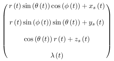
(define ((sf->rf qs) state-with-force)
  (let* ((extract (extract-particle 3))

         (p (extract state-with-force 0))
         (t (time p))
         (q (coordinate p))

         (lambd (ref (coordinate
                      state-with-force) 3))

         (r (ref q 0))
         (theta (ref q 1))
         (phi (ref q 2))

         (xs (ref qs 0))
         (ys (ref qs 1))
         (zs (ref qs 2))

         (x (+ (xs t)
               (* r (sin theta) (cos phi))))
         (y (+ (ys t)
               (* r (sin theta) (sin phi))))
         (z (+ (zs t)
               (* r (cos theta)))))

    (up x y z lambd)))

(let* ((xs (literal-function 'x_s))
       (ys (literal-function 'y_s))
       (zs (literal-function 'z_s))
       (qs (up xs ys zs))
       (q (up (literal-function 'r)
              (literal-function 'theta)
              (literal-function 'phi)
              (literal-function 'lambda))))
  (show-expression
   ((compose (sf->rf qs) (Gamma q))
    't)))
(define ((F->C F) local)
  (->local (time local)
           (F local)
           (+ (((partial 0) F) local)
              (* (((partial 1) F) local)
                 (velocity local)))))

(define (L-driven m R qs U)
  (compose
   (L-rect m R qs U)
   (F->C (sf->rf qs))))
…
[guess]
— Me@2023-08-20 05:02:09 PM
.
.
2023.08.23 Wednesday (c) All rights reserved by ACHK
Structure and Interpretation of Classical Mechanics
.
A particle of mass 


~~~

(define ((KE m g R) local)
  (let ((t (time local))
        (thetadot (velocity local)))
    (* 1/2 m (square R) (square thetadot))))

(define ((PE m g R) local)
  (let ((t (time local))
        (theta (coordinate local))
        (thetadot (velocity local)))
    (- (* m g R (- 1 (cos theta))))))

(define L (- KE PE))

(show-expression
 ((L 'm 'g 'R)
  (->local 't
           'theta
           'thetadot)))

(show-expression
 (((Lagrange-equations
    (L 'm 'g 'R))
   (literal-function 'theta))
  't))

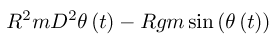
This derivation is wrong, because the constraint force is missing.
.
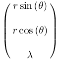
(define ((F->C F) local)
  (->local (time local)
           (F local)
           (+ (((partial 0) F) local)
              (* (((partial 1) F) local)
                 (velocity local)))))

(define (q->r local)
  (let ((q (coordinate local)))
    (let ((r (ref q 0))
          (theta (ref q 1))
          (lambd (ref q 2)))
      (let ((x (* r (sin theta)))
            (y (* r (cos theta))))
        (up x y lambd)))))

(show-expression
 (q->r
  (->local 't
           (up 'r 'theta 'lambda)
           (up 'rdot 'thetadot 'lambdadot))))
(define (KE m vx vy)
  (* 1/2 m (+ (square vx) (square vy))))

(define ((T-rect m) local)
  (let ((q (coordinate local))
        (v (velocity local)))
    (let ((xdot (ref v 0))
          (ydot (ref v 1)))
      (KE m xdot ydot))))

(show-expression
 ((T-rect 'm)
  (up 't
      (up 'x 'y 'lambda)
      (up 'xdot 'ydot 'lambdadot))))

(show-expression
 ((T-rect 'm)
  ((F->C q->r)
   (->local 't
            (up 'r 'theta 'lambda)
            (up 'rdot 'thetadot 'lambdadot)))))
(define ((U-rect g m) local)
  (let* ((q (coordinate local))
         (y (ref q 1)))
    (* g (+ (* m y)))))

(define (L-rect g m)
  (- (T-rect m) (U-rect g m)))

(define (L g m)
  (compose
   (L-rect g m) (F->C q->r)))

(show-expression
 ((L 'g 'm)
  (->local 't
           (up 'r 'theta 'lambda)
           (up 'rdot 'thetadot 'lambdadot))))
(show-expression
 (((Lagrange-equations
    (L 'g 'm))
   (up
    (literal-function 'r)
    (literal-function 'theta)
    (literal-function 'lambda)))
  't))

(define ((U-constraint R) local)
  (let* ((q (coordinate local))
         (x (ref q 0))
         (y (ref q 1))
         (lambd (ref q 2))
         (r_sq (+ (square x) (square y))))
    (* lambd (- r_sq (square R)))))

(define ((U2-constraint R) local)
  (let* ((q (coordinate local))
         (x (ref q 0))
         (y (ref q 1))
         (lambd (ref q 2))
         (r_sq (+ (square x) (square y))))
    (* lambd (- (sqrt r_sq) R))))
(define (L-rect-constraint g m R)
  (- (T-rect m) (+ (U-rect g m) (U-constraint R))))

(define (L2-rect-constraint g m R)
  (- (T-rect m) (+ (U-rect g m) (U2-constraint R))))

(show-expression
 ((L-rect-constraint 'g 'm 'R)
  ((F->C q->r)
   (->local 't
            (up 'r 'theta 'lambda)
            (up 'rdot 'thetadot 'lambdadot)))))

(show-expression
 ((L2-rect-constraint 'g 'm 'R)
  ((F->C q->r)
   (->local 't
            (up 'r 'theta 'lambda)
            (up 'rdot 'thetadot 'lambdadot)))))
(show-expression
 (((Lagrange-equations
    (compose (L-rect-constraint 'g 'm 'R) (F->C q->r)))
   (up
    (literal-function 'r)
    (literal-function 'theta)
    (literal-function 'lambda)))
  't))

(show-expression
 (((Lagrange-equations
    (compose (L2-rect-constraint 'g 'm 'R) (F->C q->r)))
   (up
    (literal-function 'r)
    (literal-function 'theta)
    (literal-function 'lambda)))
  't))
(show-expression
 (((Lagrange-equations
    (compose (L-rect-constraint 'g 'm 'R) (F->C q->r)))
   (up
    (lambda (t) 'R)
    (literal-function 'theta)
    (literal-function 'lambda)))
  't))

— Me@2023-07-12 10:00:19 PM
.
.
2023.07.13 Thursday (c) All rights reserved by ACHK
Structure and Interpretation of Classical Mechanics
.
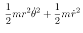
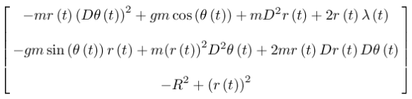
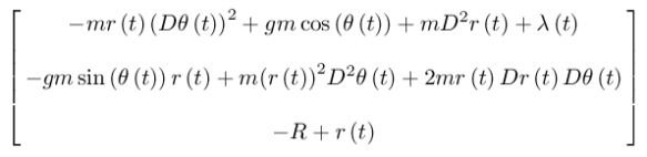
A particle of mass
~~~

.
Kinetic energy:
Potential energy:
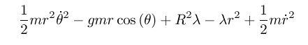
Constraint:
.
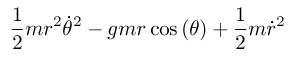
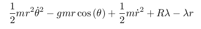
The Lagrangian:
The Lagrange equations:
.
.
.
.
By the constraint 
— Me@2023-06-25 07:47:21 PM
.
.
2023.06.28 Wednesday (c) All rights reserved by ACHK
![\displaystyle{E[F + G] = E[F] + E[G]}](https://s0.wp.com/latex.php?latex=%5Cdisplaystyle%7BE%5BF+%2B+G%5D+%3D+E%5BF%5D+%2B+E%5BG%5D%7D&bg=ffffff&fg=333333&s=1&c=20201002)
![\displaystyle{\mathcal{E}[F \circ C] = D_t (DF \circ C) \partial_2 C + DF \circ C \mathcal{E}[C]}](https://s0.wp.com/latex.php?latex=%5Cdisplaystyle%7B%5Cmathcal%7BE%7D%5BF+%5Ccirc+C%5D+%3D+D_t+%28DF+%5Ccirc+C%29+%5Cpartial_2+C+%2B+DF+%5Ccirc+C+%5Cmathcal%7BE%7D%5BC%5D%7D&bg=ffffff&fg=333333&s=1&c=20201002)
}](https://s0.wp.com/latex.php?latex=%5Cdisplaystyle%7B%5Cbar+%5CGamma+%28%5Cbar+f%29+%28t%2C+q%2C+v%2C+%5Cdots%29+%3D+%5Cbar+f+%5B%5Cmathcal%7BO%7D+%28t%2Cq%2Cv%2C+%5Cdots%29%5D%28t%29%7D&bg=ffffff&fg=333333&s=1&c=20201002)
![\displaystyle{E[L] = D_t \partial_2 L - \partial_1 L}](https://s0.wp.com/latex.php?latex=%5Cdisplaystyle%7BE%5BL%5D+%3D+D_t+%5Cpartial_2+L+-+%5Cpartial_1+L%7D&bg=ffffff&fg=333333&s=1&c=20201002)
![\displaystyle{ \begin{aligned} E[L] &= D_t \partial_2 L - \partial_1 L \\ E[F+G] &= D_t \left( \partial_2 (F+G) \right) - \partial_1 (F+G) \\ &= D_t \left( \partial_2 F+\partial_2 G \right) - (\partial_1 F+ \partial_1 G) \\ &= D_t \partial_2 F+D_t \partial_2 G - (\partial_1 F+ \partial_1 G) \\ &= D_t \partial_2 F- \partial_1 F +D_t \partial_2 G - \partial_1 G \\ &= E[F] + E[G] \\ \end{aligned} }](https://s0.wp.com/latex.php?latex=%5Cdisplaystyle%7B++%5Cbegin%7Baligned%7D++E%5BL%5D+%26%3D+D_t+%5Cpartial_2+L+-+%5Cpartial_1+L+%5C%5C+++E%5BF%2BG%5D+%26%3D+D_t+%5Cleft%28+%5Cpartial_2+%28F%2BG%29+%5Cright%29+-+%5Cpartial_1+%28F%2BG%29+%5C%5C+++%26%3D+D_t+%5Cleft%28+%5Cpartial_2+F%2B%5Cpartial_2+G+%5Cright%29+-+%28%5Cpartial_1+F%2B+%5Cpartial_1+G%29+%5C%5C+++%26%3D+D_t+%5Cpartial_2+F%2BD_t+%5Cpartial_2+G+-+%28%5Cpartial_1+F%2B+%5Cpartial_1+G%29+%5C%5C++%26%3D+D_t+%5Cpartial_2+F-+%5Cpartial_1+F+%2BD_t+%5Cpartial_2+G+-+%5Cpartial_1+G+%5C%5C+++%26%3D+E%5BF%5D+%2B+E%5BG%5D+%5C%5C++%5Cend%7Baligned%7D++%7D&bg=ffffff&fg=333333&s=1&c=20201002)
![\displaystyle{ \begin{aligned} &E[F \circ C] (t,q,v,\dots) \\ &= (D_t \partial_2 (F \circ C) - \partial_1 (F \circ C)) (t,q,v,\dots)\\ &= (D_t \partial_2 (F (C(t,q,v,\dots))) - \partial_1 (F(C(t,q,v,\dots)))) \\ \end{aligned} }](https://s0.wp.com/latex.php?latex=%5Cdisplaystyle%7B++%5Cbegin%7Baligned%7D++%26E%5BF+%5Ccirc+C%5D+%28t%2Cq%2Cv%2C%5Cdots%29+%5C%5C+++%26%3D+%28D_t+%5Cpartial_2+%28F+%5Ccirc+C%29+-+%5Cpartial_1+%28F+%5Ccirc+C%29%29+%28t%2Cq%2Cv%2C%5Cdots%29%5C%5C+++++%26%3D+%28D_t+%5Cpartial_2+%28F+%28C%28t%2Cq%2Cv%2C%5Cdots%29%29%29+-+%5Cpartial_1+%28F%28C%28t%2Cq%2Cv%2C%5Cdots%29%29%29%29+%5C%5C+++++%5Cend%7Baligned%7D++%7D&bg=ffffff&fg=333333&s=1&c=20201002)


![\displaystyle{\begin{aligned} & \left. \bar \Gamma (\bar f) \circ \Gamma [q] \right|_{t_0} \\ &= \left. \bar \Gamma (\bar f) \circ \Gamma[\mathcal{O} (t,q,v,a)](t)\right|_{t_0} \\ &= \left. \bar \Gamma (\bar f) (t, q, v, a)\right|_{t_0} \\ &= \left[ v_0 + a_0 (t-t_0) \right]_{t_0} \\ &= \cos (t_0) \\ \end{aligned}}](https://s0.wp.com/latex.php?latex=%5Cdisplaystyle%7B%5Cbegin%7Baligned%7D++++%26+%5Cleft.+%5Cbar+%5CGamma+%28%5Cbar+f%29+%5Ccirc+%5CGamma+%5Bq%5D+%5Cright%7C_%7Bt_0%7D+%5C%5C++%26%3D+%5Cleft.+%5Cbar+%5CGamma+%28%5Cbar+f%29+%5Ccirc+%5CGamma%5B%5Cmathcal%7BO%7D+%28t%2Cq%2Cv%2Ca%29%5D%28t%29%5Cright%7C_%7Bt_0%7D+%5C%5C++%26%3D+%5Cleft.+%5Cbar+%5CGamma+%28%5Cbar+f%29+%28t%2C+q%2C+v%2C+a%29%5Cright%7C_%7Bt_0%7D+%5C%5C++%26%3D+%5Cleft%5B+v_0+%2B+a_0+%28t-t_0%29+%5Cright%5D_%7Bt_0%7D+%5C%5C++%26%3D+%5Ccos+%28t_0%29+%5C%5C+++%5Cend%7Baligned%7D%7D&bg=ffffff&fg=333333&s=1&c=20201002)

![\displaystyle{\begin{aligned} & \left. \bar \Gamma (\bar g) \circ \Gamma [q] \right|_{t_0} \\ &= \left. \bar \Gamma (\bar g) \circ \Gamma[\mathcal{O} (t,q,v,a)](t)\right|_{t_0} \\ &= \left. \bar \Gamma (\bar g) (t, q, v, a)\right|_{t_0} \\ &= \left[ 0 \right]_{t_0} \\ &= 0 \\ \end{aligned}}](https://s0.wp.com/latex.php?latex=%5Cdisplaystyle%7B%5Cbegin%7Baligned%7D++++%26+%5Cleft.+%5Cbar+%5CGamma+%28%5Cbar+g%29+%5Ccirc+%5CGamma+%5Bq%5D+%5Cright%7C_%7Bt_0%7D+%5C%5C++%26%3D+%5Cleft.+%5Cbar+%5CGamma+%28%5Cbar+g%29+%5Ccirc+%5CGamma%5B%5Cmathcal%7BO%7D+%28t%2Cq%2Cv%2Ca%29%5D%28t%29%5Cright%7C_%7Bt_0%7D+%5C%5C++%26%3D+%5Cleft.+%5Cbar+%5CGamma+%28%5Cbar+g%29+%28t%2C+q%2C+v%2C+a%29%5Cright%7C_%7Bt_0%7D+%5C%5C++%26%3D+%5Cleft%5B+0+%5Cright%5D_%7Bt_0%7D+%5C%5C++%26%3D+0+%5C%5C+++%5Cend%7Baligned%7D%7D&bg=ffffff&fg=333333&s=1&c=20201002)


}](https://s0.wp.com/latex.php?latex=%5Cdisplaystyle%7B%28t%2Cq%2Cv%2C%5Ccdots%2C+q%5E%7B%28n%29%7D%29+%3D+%5CGamma%5B%5Cmathcal%7BO%7D+%28t%2Cq%2Cv%2C+%5Ccdots%2C+q%5E%7B%28n%29%7D%5D%28t%29%7D&bg=ffffff&fg=333333&s=1&c=20201002)
![\displaystyle{\begin{aligned} f (t, q(t), v(t), \cdots, q^{(n)}(t)) &= f(\Gamma[q])(t) \\ \bar \Gamma (\bar f) (t, q(t), v(t), \cdots, q^{(n)}(t)) &= \bar f [q](t) \\ \end{aligned}}](https://s0.wp.com/latex.php?latex=%5Cdisplaystyle%7B%5Cbegin%7Baligned%7D++f+%28t%2C+q%28t%29%2C+v%28t%29%2C+%5Ccdots%2C+q%5E%7B%28n%29%7D%28t%29%29+%26%3D+f%28%5CGamma%5Bq%5D%29%28t%29+%5C%5C++%5Cbar+%5CGamma+%28%5Cbar+f%29+%28t%2C+q%28t%29%2C+v%28t%29%2C+%5Ccdots%2C+q%5E%7B%28n%29%7D%28t%29%29+%26%3D+%5Cbar+f+%5Bq%5D%28t%29+%5C%5C++%5Cend%7Baligned%7D%7D&bg=ffffff&fg=333333&s=1&c=20201002)
![\displaystyle{\begin{aligned} q &= F \circ (\Gamma[q']) \\ \bar f [q'] &= \Gamma[q] \\ &= \Gamma[F \circ \Gamma[q']] \end{aligned}}](https://s0.wp.com/latex.php?latex=%5Cdisplaystyle%7B%5Cbegin%7Baligned%7D++q+%26%3D+F+%5Ccirc+%28%5CGamma%5Bq%27%5D%29+%5C%5C++%5Cbar+f+%5Bq%27%5D+%26%3D+%5CGamma%5Bq%5D+%5C%5C++%26%3D+%5CGamma%5BF+%5Ccirc+%5CGamma%5Bq%27%5D%5D++%5Cend%7Baligned%7D%7D&bg=ffffff&fg=333333&s=1&c=20201002)

![\displaystyle{\begin{aligned} \Gamma [q] &= (t, q, v, \cdots) \\ \bar f &= f \circ \Gamma \\ \end{aligned}}](https://s0.wp.com/latex.php?latex=%5Cdisplaystyle%7B%5Cbegin%7Baligned%7D+%5CGamma+%5Bq%5D+%26%3D+%28t%2C+q%2C+v%2C+%5Ccdots%29+%5C%5C+%5Cbar+f+%26%3D+f+%5Ccirc+%5CGamma+%5C%5C+%5Cend%7Baligned%7D%7D&bg=ffffff&fg=333333&s=1&c=20201002)
![\displaystyle{\begin{aligned} f (t, q(t), v(t), \cdots, q^{(n)}(t)) &= f(\Gamma[q])(t) \\ \bar \Gamma (\bar f) (t, q(t), v(t), \cdots, q^{(n)}(t)) &= \bar f [q](t) \\ \end{aligned}}](https://s0.wp.com/latex.php?latex=%5Cdisplaystyle%7B%5Cbegin%7Baligned%7D++f+%28t%2C+q%28t%29%2C+v%28t%29%2C+%5Ccdots%2C+q%5E%7B%28n%29%7D%28t%29%29+++++%26%3D+f%28%5CGamma%5Bq%5D%29%28t%29+%5C%5C+++++%5Cbar+%5CGamma+%28%5Cbar+f%29+%28t%2C+q%28t%29%2C+v%28t%29%2C+%5Ccdots%2C+q%5E%7B%28n%29%7D%28t%29%29+++++%26%3D+%5Cbar+f+%5Bq%5D%28t%29+%5C%5C+++++%5Cend%7Baligned%7D%7D&bg=ffffff&fg=333333&s=1&c=20201002)
![\displaystyle{\begin{aligned} L' \circ \Gamma[q'] &= L \circ \Gamma [q] \\ \Gamma[q] &= C \circ \Gamma[q'] \\ L' &= L \circ C \\ \end{aligned}}](https://s0.wp.com/latex.php?latex=%5Cdisplaystyle%7B%5Cbegin%7Baligned%7D+++L%27+%5Ccirc+%5CGamma%5Bq%27%5D+%26%3D+L+%5Ccirc+%5CGamma+%5Bq%5D+%5C%5C+++%5CGamma%5Bq%5D+%26%3D+C+%5Ccirc+%5CGamma%5Bq%27%5D+%5C%5C+++L%27+%26%3D+L+%5Ccirc+C+%5C%5C+++%5Cend%7Baligned%7D%7D&bg=ffffff&fg=333333&s=1&c=20201002)
![\displaystyle{\begin{aligned} \Gamma[q] &= C \circ \Gamma[q'] \\ (t, x, v, \cdots) &= (t, F(t,x'), \partial_0 F(t, x') + \partial_1 F(t, x') v', \cdots) \\ \end{aligned}}](https://s0.wp.com/latex.php?latex=%5Cdisplaystyle%7B%5Cbegin%7Baligned%7D+++%5CGamma%5Bq%5D+%26%3D+C+%5Ccirc+%5CGamma%5Bq%27%5D+%5C%5C+++%28t%2C+x%2C+v%2C+%5Ccdots%29+%26%3D+%28t%2C+F%28t%2Cx%27%29%2C+%5Cpartial_0+F%28t%2C+x%27%29+%2B+%5Cpartial_1+F%28t%2C+x%27%29+v%27%2C+%5Ccdots%29+%5C%5C++++%5Cend%7Baligned%7D%7D&bg=ffffff&fg=333333&s=1&c=20201002)
![\displaystyle{\begin{aligned} f (t, q(t), v(t), \cdots, q^{(n)}(t)) &= f (t, q, v, \cdots, q^{(n)})(t) \\ &= f(\Gamma[q])(t) \\ &= f \circ \Gamma[q](t) \\ &= \bar f [q](t) \\ \bar \Gamma (\bar f) (t, q(t), v(t), \cdots, q^{(n)}(t)) &= \bar f [q](t) \\ \end{aligned}}](https://s0.wp.com/latex.php?latex=%5Cdisplaystyle%7B%5Cbegin%7Baligned%7D++f+%28t%2C+q%28t%29%2C+v%28t%29%2C+%5Ccdots%2C+q%5E%7B%28n%29%7D%28t%29%29+++%26%3D+f+%28t%2C+q%2C+v%2C+%5Ccdots%2C+q%5E%7B%28n%29%7D%29%28t%29+%5C%5C+++%26%3D+f%28%5CGamma%5Bq%5D%29%28t%29+%5C%5C+++%26%3D+f+%5Ccirc+%5CGamma%5Bq%5D%28t%29+%5C%5C+++%26%3D+%5Cbar+f+%5Bq%5D%28t%29+%5C%5C+++%5Cbar+%5CGamma+%28%5Cbar+f%29+%28t%2C+q%28t%29%2C+v%28t%29%2C+%5Ccdots%2C+q%5E%7B%28n%29%7D%28t%29%29+++%26%3D+%5Cbar+f+%5Bq%5D%28t%29+%5C%5C+++%5Cend%7Baligned%7D%7D&bg=ffffff&fg=333333&s=1&c=20201002)

 \\ \end{aligned}}](https://s0.wp.com/latex.php?latex=%5Cdisplaystyle%7B%5Cbegin%7Baligned%7D++%5Cbar+%5CGamma+%28%5Cbar+f%29+%28t%2C+q%28t%29%2C+v%28t%29%2C+%5Ccdots%29+%26%3D+%5Cbar+f%5BO%28t%2C+q%2C+v%2C+%5Ccdots%29%5D%28t%29+%5C%5C+++%5Cend%7Baligned%7D%7D&bg=ffffff&fg=333333&s=1&c=20201002)
![\displaystyle{\begin{aligned} \Gamma [q] &= (t, q, v, \cdots) \\ \bar f &= f \circ \Gamma \\ \end{aligned}}](https://s0.wp.com/latex.php?latex=%5Cdisplaystyle%7B%5Cbegin%7Baligned%7D++%5CGamma+%5Bq%5D+%26%3D+%28t%2C+q%2C+v%2C+%5Ccdots%29+%5C%5C+++%5Cbar+f+%26%3D+f+%5Ccirc+%5CGamma+%5C%5C++%5Cend%7Baligned%7D%7D&bg=ffffff&fg=333333&s=1&c=20201002)
![\displaystyle{\begin{aligned} \Gamma [q] &= (t, q, v, \cdots, q^{(n)}) \\ &= (t, q^{(0)}, q^{(1)}, \cdots, q^{(n)}) \\ \end{aligned}}](https://s0.wp.com/latex.php?latex=%5Cdisplaystyle%7B%5Cbegin%7Baligned%7D++%5CGamma+%5Bq%5D+%26%3D+%28t%2C+q%2C+v%2C+%5Ccdots%2C+q%5E%7B%28n%29%7D%29+%5C%5C+++%26%3D+%28t%2C+q%5E%7B%280%29%7D%2C+q%5E%7B%281%29%7D%2C+%5Ccdots%2C+q%5E%7B%28n%29%7D%29+%5C%5C+++%5Cend%7Baligned%7D%7D&bg=ffffff&fg=333333&s=1&c=20201002)


![\displaystyle{\begin{aligned} T(r(t), \theta(t)) &= \frac{1}{2} m \left( v_x^2 + v_y^2 \right) \\ &= \frac{1}{2} m \left[ \left( \frac{d}{dt} r \sin \theta \right)^2 + \left( \frac{d}{dt} r \cos \theta \right)^2 \right] \\ &= \frac{1}{2} m \left[ \left( \dot r \sin \theta + r \dot \theta \cos \theta \right)^2 + \left( \dot r \cos \theta - r \dot \theta \sin \theta \right)^2 \right] \\ &= \frac{1}{2} m \left[ \dot r^2 + r^2 \dot \theta^2 \right] \\ \end{aligned}}](https://s0.wp.com/latex.php?latex=%5Cdisplaystyle%7B%5Cbegin%7Baligned%7D++++++++++T%28r%28t%29%2C+%5Ctheta%28t%29%29+++++%26%3D+%5Cfrac%7B1%7D%7B2%7D+m+%5Cleft%28+v_x%5E2+%2B+v_y%5E2+%5Cright%29+%5C%5C+++++++++%26%3D+%5Cfrac%7B1%7D%7B2%7D+m+%5Cleft%5B+%5Cleft%28+%5Cfrac%7Bd%7D%7Bdt%7D+r+%5Csin+%5Ctheta+%5Cright%29%5E2+%2B+%5Cleft%28+%5Cfrac%7Bd%7D%7Bdt%7D+r+%5Ccos+%5Ctheta+%5Cright%29%5E2+%5Cright%5D+%5C%5C+++++++++%26%3D+%5Cfrac%7B1%7D%7B2%7D+m+%5Cleft%5B+++++%5Cleft%28+%5Cdot+r+%5Csin+%5Ctheta+%2B+r+%5Cdot+%5Ctheta+%5Ccos+%5Ctheta+%5Cright%29%5E2+++%2B+%5Cleft%28+%5Cdot+r+%5Ccos+%5Ctheta+-+r+%5Cdot+%5Ctheta+%5Csin+%5Ctheta+%5Cright%29%5E2+++%5Cright%5D+%5C%5C+++++++++%26%3D+%5Cfrac%7B1%7D%7B2%7D+m+%5Cleft%5B+%5Cdot+r%5E2+%2B+r%5E2+%5Cdot+%5Ctheta%5E2++%5Cright%5D+%5C%5C+++++++++++%5Cend%7Baligned%7D%7D&bg=ffffff&fg=333333&s=1&c=20201002)


You must be logged in to post a comment.