
— Me@2022-04-06 10:02:58 AM
.
.
2022.04.06 Wednesday (c) All rights reserved by ACHK

— Me@2022-04-06 10:02:58 AM
.
.
2022.04.06 Wednesday (c) All rights reserved by ACHK
Ex 1.22 Driven pendulum, 3.2
Structure and Interpretation of Classical Mechanics
.
Find the tension in an undriven planar pendulum.
~~~
[guess]
(define ((q->r x_s y_s l) local)
  (let* ((q (coordinate local))
         (t (time local))
         (theta (ref q 0))
         (c (ref q 1))
         (F (ref q 2)))
    (up (+ (x_s t) (* c (sin theta)))
        (- (y_s t) (* c (cos theta)))
        F)))

(let* ((xs (literal-function 'x_s))
       (ys (literal-function 'y_s))
       (q (up (literal-function 'theta)
              (literal-function 'c)
              (literal-function 'F))))
  (show-expression ((compose (q->r xs ys 'l) (Gamma q)) 't)))

(define (L-theta m l x_s y_s U)
  (compose
   (L-driven-free m l x_s y_s U) (F->C (q->r x_s y_s l))))

(let* ((U (U-gravity 'g 'm))
       (xs (literal-function 'x_s))
       (ys (literal-function 'y_s))
       (q (up (literal-function 'theta)
              (literal-function 'c)
              (literal-function 'F)))
       (L (L-theta 'm 'l xs ys U)))
  (show-expression (L ((Gamma q) 't))))
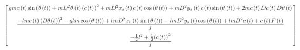
(/
 (+ (* l m ((D x_s) t) (c t) ((D theta) t) (cos (theta t)))
    (* 1/2 l m (expt (c t) 2) (expt ((D theta) t) 2))
    (* l m (c t) ((D theta) t) (sin (theta t)) ((D y_s) t))
    (* g l m (c t) (cos (theta t)))
    (* l m ((D x_s) t) ((D c) t) (sin (theta t)))
    (* -1 l m ((D c) t) (cos (theta t)) ((D y_s) t))
    (* -1 g l m (y_s t))
    (* 1/2 l m (expt ((D x_s) t) 2))
    (* 1/2 l m (expt ((D c) t) 2))
    (* 1/2 l m (expt ((D y_s) t) 2))
    (* 1/2 (expt l 2) (F t))
    (* -1/2 (expt (c t) 2) (F t)))
 l)
(let* ((U (U-gravity 'g 'm))
       (xs (literal-function 'x_s))
       (ys (literal-function 'y_s))
       (q (up (literal-function 'theta)
              (literal-function 'c)
              (literal-function 'F)))
       (L (L-theta 'm 'l xs ys U)))
  (show-expression (((Lagrange-equations L) q) 't)))
.
(let* ((U (U-gravity 'g 'm))
       (xs (lambda (t) 0))
       (ys (lambda (t) 'l))
       (q (up (literal-function 'theta)
              (lambda (t) 'l)
              (literal-function 'F)))
       (L (L-theta 'm 'l xs ys U)))
  (show-expression (((Lagrange-equations L) q) 't)))

.
.
[guess]
— Me@2022-04-05 04:16:51 PM
.
.
2022.04.05 Tuesday (c) All rights reserved by ACHK
Comparison of pictures
The Heisenberg picture is closest to classical Hamiltonian mechanics (for example, the commutators appearing in the above equations directly correspond to classical Poisson brackets). The Schrödinger picture, the preferred formulation in introductory texts, is easy to visualize in terms of Hilbert space rotations of state vectors, although it lacks natural generalization to Lorentz invariant systems. The Dirac picture is most useful in nonstationary and covariant perturbation theory, so it is suited to quantum field theory and many-body physics.
Summary comparison of evolutions
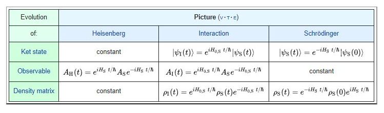
— Wikipedia on Dynamical pictures
.
.
2022.04.05 Tuesday ACHK
外在世界是地獄,心中宇宙是天堂;把知識和想像化成現實,就是把地獄天堂化。
— Me@2011.10.05
.
.
2022.04.04 Monday (c) All rights reserved by ACHK
這段改編自 2021 年 12 月 9 日的對話。
.
如果你將來遇到,一個你心儀對象的話,千萬不要以為,她一定是你未來太太。亦即是話,即使是「一見鍾情」,那也只是感覺,未必反映實情;「兩見如何」還要相處過才知道。
幾十年前,我曾經遇到,一位心儀的女士。我與她有著,電影《情留半天》級數的對話。她也對我有意思。我怎麼知道呢?
當時我煩惱著,她會否已有男朋友。但是,我又不好意思問。反而,她有天突然問我,有沒有女朋友。
.
如果可以定期見面,我們理應可以,自然發展成情侶。
.
不幸,她有著關鍵的缺點,而我又改變不到。 例如,她會連續五次失約。
— Me@2022-04-02 04:39:11 PM
.
.
2022.04.03 Sunday (c) All rights reserved by ACHK

求知若飢 虛懷若愚
— Steve Jobs
.
.
2022.04.01 Friday (c) All rights reserved by ACHK
A First Course in String Theory
.
Verify that 
~~~
Eq. (3.8):
Eq. (3.10):
.
— Me@2022-04-01 03:34:28 PM
.
.
2022.04.01 Friday (c) All rights reserved by ACHK
![\displaystyle{F(t) = l m \left[D \theta(t)\right]^2 + g m \cos \theta(t)}](https://s0.wp.com/latex.php?latex=%5Cdisplaystyle%7BF%28t%29+%3D+l+m+%5Cleft%5BD+%5Ctheta%28t%29%5Cright%5D%5E2+%2B+g+m+%5Ccos+%5Ctheta%28t%29%7D&bg=ffffff&fg=333333&s=0&c=20201002)


You must be logged in to post a comment.