3.6 Analytic continuation for gamma function, 6

Posted on July 30, 2024 by rpflee

A First Course in String Theory

Residues

The behavior for non-positive $\displaystyle{z}$ is more intricate. Euler’s integral does not converge for $\displaystyle{\Re (z)\leq 0}$ , but the function it defines in the positive complex half-plane has a unique analytic continuation to the negative half-plane. One way to find that analytic continuation is to use Euler’s integral for positive arguments and extend the domain to negative numbers by repeated application of the recurrence formula,

$\displaystyle{\Gamma (z)={\frac {\Gamma (z+n+1)}{z(z+1)\cdots (z+n)}}}$ ,

choosing $\displaystyle{n}$ such that $\displaystyle{z+n}$ is positive. The product in the denominator is zero when $\displaystyle{z}$ equals any of the integers $\displaystyle{0,-1,-2,\ldots}$ . Thus, the gamma function must be undefined at those points to avoid division by zero; it is a meromorphic function with simple poles at the non-positive integers.

— Wikipedia on Gamma function

2024.07.30 Tuesday ACHK

Quantum encryption

Posted on July 30, 2024 by rpflee

An important and unique property of quantum key distribution is the ability of the two communicating users to detect the presence of any third party trying to gain knowledge of the key. This results from a fundamental aspect of quantum mechanics: the process of measuring a quantum system in general disturbs the system. A third party trying to eavesdrop on the key must in some way measure it, thus introducing detectable anomalies.

— Wikipedia on Quantum key distribution

The common language of quantum mechanics is convenient but not accurate:

Eavesdropping would cause the collapse of the wave function, so Alice and Bob must be aware of it.

The accurate language:

A wave function encodes the probability distribution of various possible experimental outcomes of a system. In other words, the wave function is a property of the system (the experimental setup), encompassing the experimental operations, including measurements.

To eavesdrop, Eve has to add an extra detector to the system. Thus, the system is altered (replaced). So the probability distribution is no longer that of the original system. That is the meaning of “collapse of the wave function”.

— Me@2024-06-19 02:17:35 PM

Context

Posted on July 24, 2024 by rpflee

~ con text

~ what puts the texts together

— Me@2015-12-11 07:16:47 AM

Amazing Gags 9

Posted on July 22, 2024 by rpflee

這段改編自 2010 年 4 月 24 日的對話。

If you’re good at something, never do it for free.

— The Dark Knight

「搞 gag」（弄笑話）要成功的其中一個先決條件是，容許失敗。

不許失敗的話，就沒有人膽敢嘗試。

作為聽眾，遇到冷笑話時，合理的反應是，不要笑。

但部分人卻會，立刻大聲指責，彷彿你是他的殺父仇人般。

聽眾之中，本身不懂講笑話的人，往往把你，責怪得最重。

合情合理之人，不會在別人沒有惡意的情況下，尖酸刻薄。

不應對尖酸刻薄的人，主動表達善意。

嘗試搞 gag，是善意的一種。

— Me@2024-07-20 05:54:18 PM

World Cup 94, 2

Posted on July 18, 2024 by rpflee

Find the sum of the digits in the number $\displaystyle{100!}$ .

import Data.Char ( digitToInt )

p_20 = sum
       $ map digitToInt
       $ show $ product [1..100]

λ> p_20
648

— Haskell official

— Me@2024-07-17 03:44:42 PM

3 Vector Fields and One-Form Fields, 2.3

Posted on July 13, 2024 by rpflee

Functional Differential Geometry

p. 21

…

3.2

… $\displaystyle{ \textbf{v}(\text{f})(\textbf{m})}$ is the direction derivative of the function $\displaystyle{\text{f}}$ at the point $\displaystyle{ \textbf{m} }$ .

Note that it is not the ordinary directional derivative.

3.2.1

Instead, the ordinary directional derivative is

$\displaystyle{(Df(x)) \Delta x}$

$\displaystyle{\begin{aligned} D_{\mathbf{v}}(f) &= \frac{\left(\delta f\right)_{\mathbf{v}}}{|\mathbf{v}|} &= \left(\nabla f\right) \cdot \hat{\mathbf{v}} \\ \end{aligned}}$

3.2.2

The first generalization of directional derivative is replacing $\displaystyle{\Delta x}$ , a vector independent of $\displaystyle{x}$ , with $\displaystyle{b(x)}$ , a vector function of $\displaystyle{x}$ .

3.2.3

~~The second generalization of directional derivative is replacing $\displaystyle{D}$ or $\displaystyle{\nabla}$ with $\displaystyle{\textbf{v}}$ , which is a vector function chosen by you.~~

In differential geometry, a vector is an operator that takes directional derivatives of manifold functions at its anchor point.

The directional derivative of a scalar function $f$ with respect to a vector $\displaystyle{\mathbf{v}}$ at a point (e.g., position) $\displaystyle{\mathbf{x}}$ may be denoted by any of the following:

$\displaystyle{\begin{aligned} \nabla _{\mathbf {v} }{f}(\mathbf {x} ) &=f'_{\mathbf {v} }(\mathbf {x} )=D_{\mathbf {v} }f(\mathbf {x} )=Df(\mathbf {x} )(\mathbf {v} ) \\ &=\partial _{\mathbf {v} }f(\mathbf {x} )=\mathbf {v} \cdot {\nabla f(\mathbf {x} )}=\mathbf {v} \cdot {\frac {\partial f(\mathbf {x} )}{\partial \mathbf {x} }}.\end{aligned}}$

…

Let $\displaystyle{\textit{M}}$ be a differentiable manifold and $\displaystyle{\mathbf{p}}$ a point of $\displaystyle{\textit{M}}$ .

Suppose that $\displaystyle{f}$ is a function defined in a neighborhood of $\displaystyle{\mathbf{p}}$ , and differentiable at $\displaystyle{\mathbf{p}}$ .

If $\displaystyle{\mathbf{v}}$ is a tangent vector to $\displaystyle{\textit{M}}$ at $\displaystyle{\mathbf{p}}$ , then the directional derivative of $\displaystyle{f}$ along $\displaystyle{\mathbf{v}}$ , denoted variously as $\displaystyle{df(\mathbf{v})}$ (see Exterior derivative), $\displaystyle{\nabla_{\mathbf {v} }f(\mathbf {p} )}$ (see Covariant derivative), $\displaystyle{L_{\mathbf {v} }f(\mathbf {p} )}$ (see Lie derivative), or $\displaystyle{ {\mathbf {v} }_{\mathbf {p} }(f)}$ (see Tangent space § Definition via derivations), can be defined as follows.

Let $\displaystyle{\gamma: [-1, 1] \to M}$ be a differentiable curve with $\displaystyle{\gamma(0) = \mathbf{p}}$ and $\displaystyle{\gamma'(0) = \mathbf{v}}$ . Then the directional derivative is defined by

$\displaystyle{\nabla _{\mathbf {v} }f(\mathbf {p} )=\left.{\frac {d}{d\tau }}f\circ \gamma (\tau )\right|_{\tau =0}.}$

This definition can be proven independent of the choice of $\displaystyle{\gamma}$ , provided $\displaystyle{\gamma}$ is selected in the prescribed manner so that $\displaystyle{\gamma(0) = \mathbf{p}}$ and $\displaystyle{\gamma'(0) = \mathbf{v}}$ .

— Wikipedia on Directional derivative

Tangent vectors as directional derivatives

Another way to think about tangent vectors is as directional derivatives. Given a vector $\displaystyle{v}$ in $\displaystyle{ \mathbb {R} ^{n}}$ , one defines the corresponding directional derivative at a point $\displaystyle{ x\in \mathbb {R} ^{n}}$ by

$\displaystyle{ \forall f\in {C^{\infty }}(\mathbb {R} ^{n}):\qquad (D_{v}f)(x):=\left.{\frac {\mathrm {d} }{\mathrm {d} {t}}}[f(x+tv)]\right|_{t=0}=\sum _{i=1}^{n}v^{i}{\frac {\partial f}{\partial x^{i}}}(x).}$

This map is naturally a derivation at $\displaystyle{ x }$ . Furthermore, every derivation at a point in $\mathbb {R} ^{n}$ is of this form. Hence, there is a one-to-one correspondence between vectors (thought of as tangent vectors at a point) and derivations at a point.

— Wikipedia on Tangent space

4. In a more user-friendly language:

$\displaystyle{ \begin{aligned} \textbf{v}(\textbf{f})(\textbf{m}) &= D_b(f)(x) \\ \end{aligned} }$

$\displaystyle{ \begin{aligned} b^i_{\chi, \mathbf{v}} (x) &= \mathbf{v}(\chi^i) \circ \chi^{-1} (x) \\ &= \mathbf{v}(\chi^i) (\mathbf{m}) \\ &= D_b(\chi^i \circ \chi^{-1})(x) \\ &= \left(\nabla (\chi^i \circ \chi^{-1}) \right)\bigg|_x \cdot \vec b\bigg|_x \\ &= \sum_j \frac{\partial}{\partial x^j}(\chi^i \circ \chi^{-1}) \bigg|_x b^j \bigg|_x \\ \end{aligned} }$

where $\displaystyle{ x = \chi (\mathbf{m}) }$ and

$\displaystyle{ \begin{aligned} x^i &= \chi^i (\mathbf{m}) \\ &= \chi^i (\chi^{-1} (\chi (\mathbf{m}))) \\ &= (\chi^i \circ \chi^{-1}) (x) \\ \end{aligned}}$

$\displaystyle{ \begin{aligned} b^i_{\chi, \mathbf{v}} (x) &= \sum_j \frac{\partial}{\partial x^j}(\chi^i \circ \chi^{-1}) \bigg|_x b^j \bigg|_x \\ &= \sum_j \frac{\partial x^i}{\partial x^j} \bigg|_x b^j \bigg|_x \\ &= \sum_j \delta^{ij} b^j \bigg|_x \\ &= b^i(x) \\ \end{aligned} }$

This is a self-consistency check.

— Me@2024-02-03 04:45:17 PM

Feynman’s Derivation of the Schrödinger Equation

Posted on July 11, 2024 by rpflee

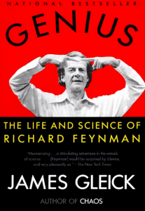
The traditional diffusion equation bore a family resemblance to the standard Schrödinger equation; the crucial difference lay in a single exponent where the quantum mechanical version was an imaginary factor, $i$ . Lacking that $i$ , diffusion was motion without inertia, motion without momentum. Individual molecules of perfume carry inertia, but their aggregate wafting through air, the sum of innumerable random collisions, does not. With the $i$ , quantum mechanics could incorporate inertia, a particle’s memory of its past velocity. The imaginary factor in the exponent mingled velocity and time in the necessary way. In a sense, quantum mechanics was diffusion in imaginary time.

— page 175

— Genius: The Life and Science of Richard Feynman

— James Gleick

2024.07.10 Wednesday ACHK

Physics Town

continues

Monthly Archives: July 2024