Source of time asymmetry in macroscopic physical systems
Second law of thermodynamics
.
.
Physics is not about reality, but about what one can say about reality.
— Bohr
— paraphrased
.
.
Physics should deduce what an observer would observe,
not what it really is, for that would be impossible.
— Me@2018-02-02 12:15:38 AM
.
.
1. Physics is about what an observer can observe about reality.
2. Whatever an observer can observe is a consistent history.
observer ~ a consistent story
observing ~ gathering a consistent story from the quantum reality
3. Physics [relativity and quantum mechanics] is also about the consistency of results of any two observers _when_, but not before, they compare those results, observational or experimental.
4. That consistency is guaranteed because the comparison of results itself can be regarded as a physical event, which can be observed by a third observer, aka a meta observer.
Since whenever an observer can observe is consistent, the meta-observer would see that the two observers have consistent observational results.
5. Either original observers is one of the possible meta-observers, since it certainly would be witnessing the comparison process of the observation data.
— Me@2018-02-02 10:25:05 PM
.
.
.
2018.02.03 Saturday (c) All rights reserved by ACHK


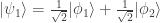


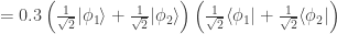
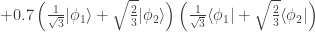


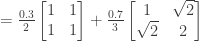


 of a density matrix in one representation can become quantum probabilities
  in another?
 or
or  , but not
  nor
nor  .
.

 個,可能的排列。亦即是話,洗牌後仍然是排列 A 的機會率,只有
  。
。
 :
: 。
。


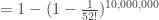
 極端接近 1。在一般情況,
 的數值還是正常時,
  會仍然極端接近 0。


 個,可能的排列。亦即是話,洗牌後仍然是排列 A 的機會率,只有
  not
not 


 radians
 represents the spatial rate of change of a scalar field along the
  direction.
 represents a displacement from point 1 to point 2 along the
  represents a displacement from point 2 to point 3 along the
  direction.
 due to the displacement
  is
is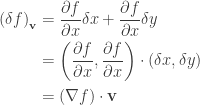
 represents the position of an object and
  is a scalar field on the
  represents the spatial rate of change of
  when the object has finished moving

 as
as

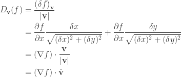
 is called directional derivative.
 is in the steepest direction.
 is chosen to be parallel to
  would be maximized.
You must be logged in to post a comment.