A First Course in String Theory
.
Physical Meaning of Virasoro Operators
The Virasoro operators are fundamental in the context of two-dimensional conformal field theory (CFT) and string theory. They arise from the study of the symmetries of two-dimensional surfaces, particularly in how these surfaces can be mapped conformally (i.e., preserving angles) onto one another.
Conformal Symmetry
The Virasoro operators are associated with the Virasoro algebra, which is an infinite-dimensional Lie algebra that extends the algebra of diffeomorphisms on a circle. This algebra captures the symmetries of two-dimensional conformal transformations. In physical terms, these transformations are crucial for understanding how physical theories behave under changes of coordinates on the worldsheet of strings or in two-dimensional quantum field theories.
Role in String Theory
In string theory, the Virasoro operators are derived from the quantization of the string’s motion. They correspond to the modes of oscillation of the string and are denoted as  . The operator
  is particularly significant because it acts as the Hamiltonian for the system, determining the energy levels of the string states. The commutation relations among these operators encode important physical information, such as the constraints on physical states (the Virasoro constraints) that must be satisfied for a consistent theory.
Physical States and Constraints
The Virasoro constraints arise from the requirement that physical states must be invariant under the action of the Virasoro operators. This leads to the notion of physical states in the theory, which are those that satisfy the condition  for
for  . This condition ensures that the states are not affected by the higher modes of the Virasoro algebra, which correspond to unphysical degrees of freedom.
Applications in CFT
In the context of conformal field theory, the Virasoro operators play a crucial role in the conformal bootstrap approach, where they help in constructing correlation functions and understanding the structure of the theory. The Virasoro conformal blocks, which are special functions derived from these operators, are essential for calculating observables in CFTs.
Summary
In summary, the Virasoro operators are central to the mathematical formulation of two-dimensional conformal field theories and string theory. They encapsulate the symmetries of these theories, dictate the physical state conditions, and facilitate the computation of physical observables. Their significance extends beyond mathematics into the core of theoretical physics, influencing our understanding of fundamental interactions and the structure of spacetime.
— AI
.
.
2024.09.08 Sunday ACHK

![[(\dot X^I - X^{I'}) (\tau, \sigma), (\dot X^J - X^{J'})(\tau, \sigma')] = - 4 \pi \alpha' i \eta^{IJ} \frac{d}{d \sigma} \delta(\sigma - \sigma')](https://s0.wp.com/latex.php?latex=%5B%28%5Cdot+X%5EI+-+X%5E%7BI%27%7D%29+%28%5Ctau%2C+%5Csigma%29%2C+%28%5Cdot+X%5EJ+-+X%5E%7BJ%27%7D%29%28%5Ctau%2C+%5Csigma%27%29%5D+%3D+-+4+%5Cpi+%5Calpha%27+i+%5Ceta%5E%7BIJ%7D+%5Cfrac%7Bd%7D%7Bd+%5Csigma%7D+%5Cdelta%28%5Csigma+-+%5Csigma%27%29&bg=ffffff&fg=333333&s=1&c=20201002)
![\left[ \alpha_m^I, \alpha_n^J \right] = m \delta_{m+n, 0} \eta^{IJ}](https://s0.wp.com/latex.php?latex=%5Cleft%5B+%5Calpha_m%5EI%2C+%5Calpha_n%5EJ+%5Cright%5D+%3D+m+%5Cdelta_%7Bm%2Bn%2C+0%7D+%5Ceta%5E%7BIJ%7D+&bg=ffffff&fg=333333&s=1&c=20201002)


![\displaystyle{\begin{aligned} \left[(\dot X^I - X^{I'}) (\tau, \sigma), (\dot X^J - X^{J'})(\tau, \sigma')\right] &= - 4 \pi \alpha' i \eta^{IJ} \frac{d}{d \sigma} \delta(\sigma - \sigma') \\ \left[ \sqrt{2 \alpha'} \sum_{m \in \mathbb{Z}} \alpha_m^I e^{-i m (\tau - \sigma)}, \sqrt{2 \alpha'} \sum_{n \in \mathbb{Z}} \alpha_n^J e^{-i n (\tau - \sigma')} \right] &= - 4 \pi \alpha' i \eta^{IJ} \frac{d}{d \sigma} \delta(\sigma - \sigma') \\ \sum_{m \in \mathbb{Z}} \sum_{n \in \mathbb{Z}} e^{-i m (\tau - \sigma)} e^{-i n (\tau - \sigma')} \left[ \alpha_m^I , \alpha_n^J \right] &= - 2 \pi i \eta^{IJ} \frac{d}{d \sigma} \delta(\sigma - \sigma') \\ \end{aligned}}](https://s0.wp.com/latex.php?latex=%5Cdisplaystyle%7B%5Cbegin%7Baligned%7D++++%5Cleft%5B%28%5Cdot+X%5EI+-+X%5E%7BI%27%7D%29+%28%5Ctau%2C+%5Csigma%29%2C+%28%5Cdot+X%5EJ+-+X%5E%7BJ%27%7D%29%28%5Ctau%2C+%5Csigma%27%29%5Cright%5D+%26%3D+-+4+%5Cpi+%5Calpha%27+i+%5Ceta%5E%7BIJ%7D+%5Cfrac%7Bd%7D%7Bd+%5Csigma%7D+%5Cdelta%28%5Csigma+-+%5Csigma%27%29+%5C%5C++++%5Cleft%5B+%5Csqrt%7B2+%5Calpha%27%7D+%5Csum_%7Bm+%5Cin+%5Cmathbb%7BZ%7D%7D+%5Calpha_m%5EI+e%5E%7B-i+m+%28%5Ctau+-+%5Csigma%29%7D%2C+%5Csqrt%7B2+%5Calpha%27%7D+%5Csum_%7Bn+%5Cin+%5Cmathbb%7BZ%7D%7D+%5Calpha_n%5EJ+e%5E%7B-i+n+%28%5Ctau+-+%5Csigma%27%29%7D+%5Cright%5D+%26%3D+-+4+%5Cpi+%5Calpha%27+i+%5Ceta%5E%7BIJ%7D+%5Cfrac%7Bd%7D%7Bd+%5Csigma%7D+%5Cdelta%28%5Csigma+-+%5Csigma%27%29+%5C%5C++++%5Csum_%7Bm+%5Cin+%5Cmathbb%7BZ%7D%7D+%5Csum_%7Bn+%5Cin+%5Cmathbb%7BZ%7D%7D+e%5E%7B-i+m+%28%5Ctau+-+%5Csigma%29%7D+e%5E%7B-i+n+%28%5Ctau+-+%5Csigma%27%29%7D+%5Cleft%5B+%5Calpha_m%5EI+%2C+%5Calpha_n%5EJ+%5Cright%5D+%26%3D+-+2+%5Cpi+i+%5Ceta%5E%7BIJ%7D+%5Cfrac%7Bd%7D%7Bd+%5Csigma%7D+%5Cdelta%28%5Csigma+-+%5Csigma%27%29+%5C%5C++++++%5Cend%7Baligned%7D%7D&bg=ffffff&fg=333333&s=1&c=20201002)
![\displaystyle{\begin{aligned} \frac{1}{2 \pi} \int_0^{2 \pi} d \sigma e^{iq\sigma} \sum_{m \in \mathbb{Z}} \sum_{n \in \mathbb{Z}} e^{-i (m+n) \tau} e^{i m \sigma} e^{i n \sigma'} \left[ \alpha_m^I , \alpha_n^J \right] &= - 2 \pi i \eta^{IJ} \frac{1}{2 \pi} \int_0^{2 \pi} d \sigma e^{iq\sigma} \frac{d}{d \sigma} \delta(\sigma - \sigma') \\ \end{aligned}}](https://s0.wp.com/latex.php?latex=%5Cdisplaystyle%7B%5Cbegin%7Baligned%7D++++%5Cfrac%7B1%7D%7B2+%5Cpi%7D+%5Cint_0%5E%7B2+%5Cpi%7D+d+%5Csigma+e%5E%7Biq%5Csigma%7D+%5Csum_%7Bm+%5Cin+%5Cmathbb%7BZ%7D%7D+%5Csum_%7Bn+%5Cin+%5Cmathbb%7BZ%7D%7D+e%5E%7B-i+%28m%2Bn%29+%5Ctau%7D+e%5E%7Bi+m+%5Csigma%7D+e%5E%7Bi+n+%5Csigma%27%7D+%5Cleft%5B+%5Calpha_m%5EI+%2C+%5Calpha_n%5EJ+%5Cright%5D+%26%3D+-+2+%5Cpi+i+%5Ceta%5E%7BIJ%7D+++%5Cfrac%7B1%7D%7B2+%5Cpi%7D+%5Cint_0%5E%7B2+%5Cpi%7D+d+%5Csigma+e%5E%7Biq%5Csigma%7D+%5Cfrac%7Bd%7D%7Bd+%5Csigma%7D+%5Cdelta%28%5Csigma+-+%5Csigma%27%29+%5C%5C+++++%5Cend%7Baligned%7D%7D&bg=ffffff&fg=333333&s=1&c=20201002)
![\displaystyle{\begin{aligned} \sum_{n \in \mathbb{Z}} e^{-i (-q+n) \tau} e^{i n \sigma'} \left[ \alpha_{-q}^I , \alpha_n^J \right] &= - i \eta^{IJ} \left[ \delta(2 \pi - \sigma') - \delta(0 - \sigma') - iq \int_0^{2 \pi} \delta (\sigma - \sigma') e^{i q \sigma} d\sigma \right] \\ \sum_{n \in \mathbb{Z}} e^{-i (-q+n) \tau} e^{i n \sigma'} \left[ \alpha_{-q}^I , \alpha_n^J \right]&= - i \eta^{IJ} \left[ \delta(2 \pi - \sigma') - \delta(0 - \sigma') - iq e^{i q \sigma'} \right] \\ \end{aligned}}](https://s0.wp.com/latex.php?latex=%5Cdisplaystyle%7B%5Cbegin%7Baligned%7D++++%5Csum_%7Bn+%5Cin+%5Cmathbb%7BZ%7D%7D+e%5E%7B-i+%28-q%2Bn%29+%5Ctau%7D+e%5E%7Bi+n+%5Csigma%27%7D+%5Cleft%5B+%5Calpha_%7B-q%7D%5EI+%2C+%5Calpha_n%5EJ+%5Cright%5D+%26%3D+-+i+%5Ceta%5E%7BIJ%7D++++%5Cleft%5B+%5Cdelta%282+%5Cpi+-+%5Csigma%27%29+-+%5Cdelta%280+-+%5Csigma%27%29+-+iq+%5Cint_0%5E%7B2+%5Cpi%7D+%5Cdelta+%28%5Csigma+-+%5Csigma%27%29+e%5E%7Bi+q+%5Csigma%7D+d%5Csigma+%5Cright%5D+%5C%5C+++++%5Csum_%7Bn+%5Cin+%5Cmathbb%7BZ%7D%7D+e%5E%7B-i+%28-q%2Bn%29+%5Ctau%7D+e%5E%7Bi+n+%5Csigma%27%7D+%5Cleft%5B+%5Calpha_%7B-q%7D%5EI+%2C+%5Calpha_n%5EJ+%5Cright%5D%26%3D+-+i+%5Ceta%5E%7BIJ%7D++++%5Cleft%5B+%5Cdelta%282+%5Cpi+-+%5Csigma%27%29+-+%5Cdelta%280+-+%5Csigma%27%29+-+iq+e%5E%7Bi+q+%5Csigma%27%7D+%5Cright%5D+%5C%5C+++++++%5Cend%7Baligned%7D%7D&bg=ffffff&fg=333333&s=1&c=20201002)
![\displaystyle{\begin{aligned} \frac{1}{2 \pi} \int_0^{2 \pi} d \sigma' e^{ip\sigma'} \sum_{n \in \mathbb{Z}} e^{-i (-q+n) \tau} e^{i n \sigma'} \left[ \alpha_{-q}^I , \alpha_n^J \right]&= - i \eta^{IJ} \frac{1}{2 \pi} \int_0^{2 \pi} d \sigma' e^{ip\sigma'} \left[ \delta(2 \pi - \sigma') - \delta(0 - \sigma') - iq e^{i q \sigma'} \right] \\ \end{aligned}}](https://s0.wp.com/latex.php?latex=%5Cdisplaystyle%7B%5Cbegin%7Baligned%7D++%5Cfrac%7B1%7D%7B2+%5Cpi%7D+%5Cint_0%5E%7B2+%5Cpi%7D+d+%5Csigma%27+e%5E%7Bip%5Csigma%27%7D+%5Csum_%7Bn+%5Cin+%5Cmathbb%7BZ%7D%7D+e%5E%7B-i+%28-q%2Bn%29+%5Ctau%7D+e%5E%7Bi+n+%5Csigma%27%7D+%5Cleft%5B+%5Calpha_%7B-q%7D%5EI+%2C+%5Calpha_n%5EJ+%5Cright%5D%26%3D+-+i+%5Ceta%5E%7BIJ%7D++++++%5Cfrac%7B1%7D%7B2+%5Cpi%7D+%5Cint_0%5E%7B2+%5Cpi%7D+d+%5Csigma%27+e%5E%7Bip%5Csigma%27%7D+%5Cleft%5B+%5Cdelta%282+%5Cpi+-+%5Csigma%27%29+-+%5Cdelta%280+-+%5Csigma%27%29+-+iq+e%5E%7Bi+q+%5Csigma%27%7D+%5Cright%5D+%5C%5C+++++%5Cend%7Baligned%7D%7D&bg=ffffff&fg=333333&s=1&c=20201002)
![\displaystyle{\begin{aligned} e^{i (p+q) \tau} \left[ \alpha_{-q}^I , \alpha_{-p}^J \right]&= - \eta^{IJ} \frac{1}{2 \pi} q \int_0^{2 \pi} d \sigma' e^{ip\sigma'} e^{i q \sigma'} \\ e^{i (p+q) \tau} \left[ \alpha_{-q}^I , \alpha_{-p}^J \right]&= - \eta^{IJ} q \delta_{p+q,0} \\ \\ \\ e^{i (m+n) \tau} \left[ \alpha_{-n}^I , \alpha_{-m}^J \right]&= - n \delta_{m+n,0} \eta^{IJ} \\ \end{aligned}}](https://s0.wp.com/latex.php?latex=%5Cdisplaystyle%7B%5Cbegin%7Baligned%7D++++e%5E%7Bi+%28p%2Bq%29+%5Ctau%7D+%5Cleft%5B+%5Calpha_%7B-q%7D%5EI+%2C+%5Calpha_%7B-p%7D%5EJ+%5Cright%5D%26%3D+-+%5Ceta%5E%7BIJ%7D++++++%5Cfrac%7B1%7D%7B2+%5Cpi%7D+q+%5Cint_0%5E%7B2+%5Cpi%7D+d+%5Csigma%27+e%5E%7Bip%5Csigma%27%7D+e%5E%7Bi+q+%5Csigma%27%7D+%5C%5C++++++e%5E%7Bi+%28p%2Bq%29+%5Ctau%7D+%5Cleft%5B+%5Calpha_%7B-q%7D%5EI+%2C+%5Calpha_%7B-p%7D%5EJ+%5Cright%5D%26%3D+-+%5Ceta%5E%7BIJ%7D+++++q+%5Cdelta_%7Bp%2Bq%2C0%7D++%5C%5C+%5C%5C+%5C%5C+++++e%5E%7Bi+%28m%2Bn%29+%5Ctau%7D+%5Cleft%5B+%5Calpha_%7B-n%7D%5EI+%2C+%5Calpha_%7B-m%7D%5EJ+%5Cright%5D%26%3D+-++++n+%5Cdelta_%7Bm%2Bn%2C0%7D+%5Ceta%5E%7BIJ%7D++%5C%5C++++++%5Cend%7Baligned%7D%7D&bg=ffffff&fg=333333&s=1&c=20201002)
![[ \bar{N}^\perp, \bar{\alpha}_{- \frac{q}{2}} ] = \frac{q}{2} \bar{\alpha}_{- \frac{q}{2}}](https://s0.wp.com/latex.php?latex=%5B+%5Cbar%7BN%7D%5E%5Cperp%2C+%5Cbar%7B%5Calpha%7D_%7B-+%5Cfrac%7Bq%7D%7B2%7D%7D+%5D+%3D+%5Cfrac%7Bq%7D%7B2%7D+%5Cbar%7B%5Calpha%7D_%7B-+%5Cfrac%7Bq%7D%7B2%7D%7D&bg=ffffff&fg=333333&s=1&c=20201002) and explain why
and explain why  is properly called a number operator.
![\left[ \bar \alpha_{\frac{m}{2}}, \bar \alpha_{\frac{n}{2}} \right] = \frac{m}{2} \delta_{m+n, 0}](https://s0.wp.com/latex.php?latex=%5Cleft%5B+%5Cbar+%5Calpha_%7B%5Cfrac%7Bm%7D%7B2%7D%7D%2C+%5Cbar+%5Calpha_%7B%5Cfrac%7Bn%7D%7B2%7D%7D+%5Cright%5D+%3D+%5Cfrac%7Bm%7D%7B2%7D+%5Cdelta_%7Bm%2Bn%2C+0%7D&bg=ffffff&fg=333333&s=1&c=20201002)
![[AB,C]=A[B,C]+[A,C]B](https://s0.wp.com/latex.php?latex=%5BAB%2CC%5D%3DA%5BB%2CC%5D%2B%5BA%2CC%5DB&bg=ffffff&fg=333333&s=1&c=20201002)
![\begin{aligned} &[ \bar{N}^\perp, \bar{\alpha}_{- \frac{q}{2}} ] \\ &= \sum_{p=1}^{\infty} [ \bar \alpha^i_{-p} \bar \alpha^i_{~p}, \bar{\alpha}_{- \frac{q}{2}} ] + \sum_{k \in \mathbb{Z}^+_\text{odd}} [ \bar \alpha_{- \frac{k}{2}} \bar \alpha_{\frac{k}{2}}, \bar{\alpha}_{- \frac{q}{2}} ] \end{aligned}](https://s0.wp.com/latex.php?latex=%5Cbegin%7Baligned%7D++%26%5B+%5Cbar%7BN%7D%5E%5Cperp%2C+%5Cbar%7B%5Calpha%7D_%7B-+%5Cfrac%7Bq%7D%7B2%7D%7D+%5D+%5C%5C++%26%3D+%5Csum_%7Bp%3D1%7D%5E%7B%5Cinfty%7D+%5B+%5Cbar+%5Calpha%5Ei_%7B-p%7D+%5Cbar+%5Calpha%5Ei_%7B%7Ep%7D%2C+%5Cbar%7B%5Calpha%7D_%7B-+%5Cfrac%7Bq%7D%7B2%7D%7D+%5D+%2B+%5Csum_%7Bk+%5Cin+%5Cmathbb%7BZ%7D%5E%2B_%5Ctext%7Bodd%7D%7D+%5B+%5Cbar+%5Calpha_%7B-+%5Cfrac%7Bk%7D%7B2%7D%7D+%5Cbar+%5Calpha_%7B%5Cfrac%7Bk%7D%7B2%7D%7D%2C+%5Cbar%7B%5Calpha%7D_%7B-+%5Cfrac%7Bq%7D%7B2%7D%7D+%5D++%5Cend%7Baligned%7D&bg=ffffff&fg=333333&s=1&c=20201002)
 ,
,![[\bar{N}^\perp, \bar{\alpha}_{- \frac{q}{2}} ] = 0](https://s0.wp.com/latex.php?latex=%5B%5Cbar%7BN%7D%5E%5Cperp%2C+%5Cbar%7B%5Calpha%7D_%7B-+%5Cfrac%7Bq%7D%7B2%7D%7D+%5D+%3D+0&bg=ffffff&fg=333333&s=1&c=20201002)
 ,
,![\begin{aligned} &[ \bar{N}^\perp, \bar{\alpha}_{- \frac{q}{2}} ] \\ &= \sum_{k \in \mathbb{Z}^+_\text{odd}}\left( \bar \alpha_{- \frac{k}{2}} [ \bar \alpha_{\frac{k}{2}}, \bar{\alpha}_{- \frac{q}{2}} ] + [ \bar \alpha_{- \frac{k}{2}}, \bar{\alpha}_{- \frac{q}{2}} ] \bar \alpha_{\frac{k}{2}} \right) \\ &= \sum_{k \in \mathbb{Z}^+_\text{odd}}\left( \bar \alpha_{- \frac{k}{2}} [ \bar \alpha_{\frac{k}{2}}, \bar{\alpha}_{- \frac{q}{2}} ] \right) + 0 \\ &= \bar \alpha_{- \frac{q}{2}} [ \bar \alpha_{\frac{q}{2}}, \bar{\alpha}_{- \frac{q}{2}} ] \\ &= \bar \alpha_{- \frac{q}{2}} \frac{q}{2} \\ \end{aligned}](https://s0.wp.com/latex.php?latex=%5Cbegin%7Baligned%7D++%26%5B+%5Cbar%7BN%7D%5E%5Cperp%2C+%5Cbar%7B%5Calpha%7D_%7B-+%5Cfrac%7Bq%7D%7B2%7D%7D+%5D+%5C%5C++%26%3D+%5Csum_%7Bk+%5Cin+%5Cmathbb%7BZ%7D%5E%2B_%5Ctext%7Bodd%7D%7D%5Cleft%28+++%5Cbar+%5Calpha_%7B-+%5Cfrac%7Bk%7D%7B2%7D%7D+%5B++%5Cbar+%5Calpha_%7B%5Cfrac%7Bk%7D%7B2%7D%7D%2C+%5Cbar%7B%5Calpha%7D_%7B-+%5Cfrac%7Bq%7D%7B2%7D%7D+%5D+++%2B+%5B+%5Cbar+%5Calpha_%7B-+%5Cfrac%7Bk%7D%7B2%7D%7D%2C+%5Cbar%7B%5Calpha%7D_%7B-+%5Cfrac%7Bq%7D%7B2%7D%7D+%5D+%5Cbar+%5Calpha_%7B%5Cfrac%7Bk%7D%7B2%7D%7D+%5Cright%29++%5C%5C++%26%3D+%5Csum_%7Bk+%5Cin+%5Cmathbb%7BZ%7D%5E%2B_%5Ctext%7Bodd%7D%7D%5Cleft%28+++%5Cbar+%5Calpha_%7B-+%5Cfrac%7Bk%7D%7B2%7D%7D+%5B++%5Cbar+%5Calpha_%7B%5Cfrac%7Bk%7D%7B2%7D%7D%2C+%5Cbar%7B%5Calpha%7D_%7B-+%5Cfrac%7Bq%7D%7B2%7D%7D+%5D+%5Cright%29++%2B+0++%5C%5C++%26%3D++++%5Cbar+%5Calpha_%7B-+%5Cfrac%7Bq%7D%7B2%7D%7D+%5B++%5Cbar+%5Calpha_%7B%5Cfrac%7Bq%7D%7B2%7D%7D%2C+%5Cbar%7B%5Calpha%7D_%7B-+%5Cfrac%7Bq%7D%7B2%7D%7D+%5D+++%5C%5C++%26%3D++++%5Cbar+%5Calpha_%7B-+%5Cfrac%7Bq%7D%7B2%7D%7D+%5Cfrac%7Bq%7D%7B2%7D++%5C%5C++%5Cend%7Baligned%7D&bg=ffffff&fg=333333&s=1&c=20201002)
 ,
,![\begin{aligned} &[ \bar{N}^\perp, \bar{\alpha}_{- \frac{q}{2}} ] \\ &= \sum_{k \in \mathbb{Z}^+_\text{odd}}\left( \bar \alpha_{- \frac{k}{2}} [ \bar \alpha_{\frac{k}{2}}, \bar{\alpha}_{- \frac{q}{2}} ] + [ \bar \alpha_{- \frac{k}{2}}, \bar{\alpha}_{- \frac{q}{2}} ] \bar \alpha_{\frac{k}{2}} \right) \\ &= 0 + \sum_{k \in \mathbb{Z}^+_\text{odd}} + [ \bar \alpha_{- \frac{k}{2}}, \bar{\alpha}_{- \frac{q}{2}} ] \bar \alpha_{\frac{k}{2}} \\ &= \frac{q}{2} \bar \alpha_{\frac{-q}{2}} \\ \end{aligned}](https://s0.wp.com/latex.php?latex=%5Cbegin%7Baligned%7D++%26%5B+%5Cbar%7BN%7D%5E%5Cperp%2C+%5Cbar%7B%5Calpha%7D_%7B-+%5Cfrac%7Bq%7D%7B2%7D%7D+%5D+%5C%5C++%26%3D+%5Csum_%7Bk+%5Cin+%5Cmathbb%7BZ%7D%5E%2B_%5Ctext%7Bodd%7D%7D%5Cleft%28+++%5Cbar+%5Calpha_%7B-+%5Cfrac%7Bk%7D%7B2%7D%7D+%5B++%5Cbar+%5Calpha_%7B%5Cfrac%7Bk%7D%7B2%7D%7D%2C+%5Cbar%7B%5Calpha%7D_%7B-+%5Cfrac%7Bq%7D%7B2%7D%7D+%5D+++%2B+%5B+%5Cbar+%5Calpha_%7B-+%5Cfrac%7Bk%7D%7B2%7D%7D%2C+%5Cbar%7B%5Calpha%7D_%7B-+%5Cfrac%7Bq%7D%7B2%7D%7D+%5D+%5Cbar+%5Calpha_%7B%5Cfrac%7Bk%7D%7B2%7D%7D+%5Cright%29++%5C%5C++%26%3D+0+%2B+%5Csum_%7Bk+%5Cin+%5Cmathbb%7BZ%7D%5E%2B_%5Ctext%7Bodd%7D%7D++%2B+%5B+%5Cbar+%5Calpha_%7B-+%5Cfrac%7Bk%7D%7B2%7D%7D%2C+%5Cbar%7B%5Calpha%7D_%7B-+%5Cfrac%7Bq%7D%7B2%7D%7D+%5D+%5Cbar+%5Calpha_%7B%5Cfrac%7Bk%7D%7B2%7D%7D+++%5C%5C++%26%3D++++%5Cfrac%7Bq%7D%7B2%7D+%5Cbar+%5Calpha_%7B%5Cfrac%7B-q%7D%7B2%7D%7D++%5C%5C++%5Cend%7Baligned%7D&bg=ffffff&fg=333333&s=1&c=20201002)
![[ \bar{N}^\perp, \cdot ]](https://s0.wp.com/latex.php?latex=%5B+%5Cbar%7BN%7D%5E%5Cperp%2C+%5Ccdot+%5D&bg=ffffff&fg=333333&s=1&c=20201002) should be.
should be. operators.

 rendering of answers yet. Instead, you can call

![\begin{aligned} \sum_{m',n'\in \mathbb{Z}_\text{odd}} e^{-i\frac{m'}{2}(\tau+\sigma)} e^{-i\frac{n'}{2}(\tau+\sigma')} \left[ \bar \alpha_{\frac{m'}{2}}, \bar \alpha_{\frac{n'}{2}} \right] &= 2 \pi i \frac{d}{d \sigma} \delta(\sigma - \sigma') \\ \end{aligned}](https://s0.wp.com/latex.php?latex=%5Cbegin%7Baligned%7D+++%5Csum_%7Bm%27%2Cn%27%5Cin+%5Cmathbb%7BZ%7D_%5Ctext%7Bodd%7D%7D+e%5E%7B-i%5Cfrac%7Bm%27%7D%7B2%7D%28%5Ctau%2B%5Csigma%29%7D+e%5E%7B-i%5Cfrac%7Bn%27%7D%7B2%7D%28%5Ctau%2B%5Csigma%27%29%7D+%5Cleft%5B+%5Cbar+%5Calpha_%7B%5Cfrac%7Bm%27%7D%7B2%7D%7D%2C+%5Cbar+%5Calpha_%7B%5Cfrac%7Bn%27%7D%7B2%7D%7D+%5Cright%5D+++%26%3D+2+%5Cpi+i+%5Cfrac%7Bd%7D%7Bd+%5Csigma%7D+%5Cdelta%28%5Csigma+-+%5Csigma%27%29+%5C%5C+++%5Cend%7Baligned%7D+&bg=ffffff&fg=333333&s=1&c=20201002)


![\begin{aligned} e^{-i\frac{m}{2}\tau} e^{-i\frac{n}{2}\tau} \left[ \cdots \right] &= i \frac{1}{2\pi} \left( - e^{i\frac{n}{2} 2 \pi} - e^{i\frac{n}{2} 0} - \int_0^{2 \pi} e^{i\frac{n}{2}\sigma} d e^{i \frac{m}{2} \sigma} \right) \\ e^{-i\frac{m+n}{2}\tau} \left[ \bar \alpha_{\frac{m}{2}}, \bar \alpha_{\frac{n}{2}} \right] &= i \frac{1}{2\pi} \left( - i\frac{m}{2} \int_0^{2 \pi} e^{i\frac{m+n}{2}\sigma} d \sigma \right) \\ e^{-i\frac{m+n}{2}\tau} \left[ \bar \alpha_{\frac{m}{2}}, \bar \alpha_{\frac{n}{2}} \right] &= i \frac{1}{2\pi} \left( - i\frac{m}{2} 2\pi \delta_{m+n,0} \right) \\ e^{-i\frac{m+n}{2}\tau} \left[ \bar \alpha_{\frac{m}{2}}, \bar \alpha_{\frac{n}{2}} \right] &= \frac{m}{2} \delta_{m+n,0} \\ \end{aligned}](https://s0.wp.com/latex.php?latex=%5Cbegin%7Baligned%7D+++++e%5E%7B-i%5Cfrac%7Bm%7D%7B2%7D%5Ctau%7D++e%5E%7B-i%5Cfrac%7Bn%7D%7B2%7D%5Ctau%7D+%5Cleft%5B+%5Ccdots+%5Cright%5D+++%26%3D+i+%5Cfrac%7B1%7D%7B2%5Cpi%7D+%5Cleft%28+-+e%5E%7Bi%5Cfrac%7Bn%7D%7B2%7D+2+%5Cpi%7D+-+e%5E%7Bi%5Cfrac%7Bn%7D%7B2%7D+0%7D++-+%5Cint_0%5E%7B2+%5Cpi%7D+e%5E%7Bi%5Cfrac%7Bn%7D%7B2%7D%5Csigma%7D+d+e%5E%7Bi+%5Cfrac%7Bm%7D%7B2%7D+%5Csigma%7D+%5Cright%29+%5C%5C++++++++e%5E%7B-i%5Cfrac%7Bm%2Bn%7D%7B2%7D%5Ctau%7D+%5Cleft%5B+%5Cbar+%5Calpha_%7B%5Cfrac%7Bm%7D%7B2%7D%7D%2C+%5Cbar+%5Calpha_%7B%5Cfrac%7Bn%7D%7B2%7D%7D+%5Cright%5D+++%26%3D+i+%5Cfrac%7B1%7D%7B2%5Cpi%7D+%5Cleft%28++-+i%5Cfrac%7Bm%7D%7B2%7D+%5Cint_0%5E%7B2+%5Cpi%7D+e%5E%7Bi%5Cfrac%7Bm%2Bn%7D%7B2%7D%5Csigma%7D+d+%5Csigma++%5Cright%29+%5C%5C++++e%5E%7B-i%5Cfrac%7Bm%2Bn%7D%7B2%7D%5Ctau%7D+%5Cleft%5B+%5Cbar+%5Calpha_%7B%5Cfrac%7Bm%7D%7B2%7D%7D%2C+%5Cbar+%5Calpha_%7B%5Cfrac%7Bn%7D%7B2%7D%7D+%5Cright%5D+++%26%3D+i+%5Cfrac%7B1%7D%7B2%5Cpi%7D+%5Cleft%28+++-+i%5Cfrac%7Bm%7D%7B2%7D+2%5Cpi+%5Cdelta_%7Bm%2Bn%2C0%7D+%5Cright%29+%5C%5C++++e%5E%7B-i%5Cfrac%7Bm%2Bn%7D%7B2%7D%5Ctau%7D+%5Cleft%5B+%5Cbar+%5Calpha_%7B%5Cfrac%7Bm%7D%7B2%7D%7D%2C+%5Cbar+%5Calpha_%7B%5Cfrac%7Bn%7D%7B2%7D%7D+%5Cright%5D+++%26%3D+%5Cfrac%7Bm%7D%7B2%7D+%5Cdelta_%7Bm%2Bn%2C0%7D++%5C%5C++++%5Cend%7Baligned%7D&bg=ffffff&fg=333333&s=1&c=20201002)
 directly from the oscillator expansion of
  .
.


 .
.


 is more intricate. Euler’s integral does not converge for
  , but the function it defines in the positive complex half-plane has a unique analytic continuation to the negative half-plane. One way to find that analytic continuation is to use Euler’s integral for positive arguments and extend the domain to negative numbers by repeated application of the recurrence formula,
 ,
, such that
  is positive. The product in the denominator is zero when
  . Thus, the gamma function must be undefined at those points to avoid division by zero; it is a meromorphic function with simple poles at the non-positive integers.
 .
.
 converges.
 converges.
 and
and  are finite,
  is also finite.
![\displaystyle{ \begin{aligned} &= \sum_{n=N+1}^\infty \frac{(-1)^n}{n!} \frac{1}{z+n} \left[ 1 - 0^{z+n} \right] \\ \end{aligned} \\ }](https://s0.wp.com/latex.php?latex=%5Cdisplaystyle%7B+%5Cbegin%7Baligned%7D+++%26%3D+%5Csum_%7Bn%3DN%2B1%7D%5E%5Cinfty+%5Cfrac%7B%28-1%29%5En%7D%7Bn%21%7D+%5Cfrac%7B1%7D%7Bz%2Bn%7D+%5Cleft%5B+1+-+0%5E%7Bz%2Bn%7D+%5Cright%5D+%5C%5C+%5Cend%7Baligned%7D+%5C%5C+%7D&bg=ffffff&fg=333333&s=1&c=20201002)
 .
.


 ,
,

 ,
,


![\displaystyle{ \begin{aligned} &\int_{0}^{1} t^{z-1} \frac{(-t)^n}{n!} dt \\ &= \frac{(-1)^n}{n!} \int_{0}^{1} t^{z+n-1} dt \\ &= \frac{(-1)^n}{n!} \frac{1}{z+n} \left[ 1 - 0^{z+n} \right] \\ \end{aligned} \\ }](https://s0.wp.com/latex.php?latex=%5Cdisplaystyle%7B++%5Cbegin%7Baligned%7D++++%26%5Cint_%7B0%7D%5E%7B1%7D+t%5E%7Bz-1%7D+%5Cfrac%7B%28-t%29%5En%7D%7Bn%21%7D+dt+%5C%5C++++%26%3D+%5Cfrac%7B%28-1%29%5En%7D%7Bn%21%7D+%5Cint_%7B0%7D%5E%7B1%7D+t%5E%7Bz%2Bn-1%7D+dt+%5C%5C++++%26%3D+%5Cfrac%7B%28-1%29%5En%7D%7Bn%21%7D+%5Cfrac%7B1%7D%7Bz%2Bn%7D+%5Cleft%5B+1+-+0%5E%7Bz%2Bn%7D+%5Cright%5D+%5C%5C++++%5Cend%7Baligned%7D+%5C%5C+%7D&bg=ffffff&fg=333333&s=1&c=20201002)
 is required. So for the overall integral
  to converge, a necessary condition is
 ,
, and any real
  ,
,

 :
:
 such that
  and
and  ,
, ,
,
![\displaystyle{ \begin{aligned} \int_1^\infty t^{x-1}e^{-t} dt &\le r! \int_1^\infty t^{-2} dt = - r! [ t^{-1} ]_1^\infty = r! \\ \end{aligned} \\ }](https://s0.wp.com/latex.php?latex=%5Cdisplaystyle%7B++%5Cbegin%7Baligned%7D++++%5Cint_1%5E%5Cinfty+t%5E%7Bx-1%7De%5E%7B-t%7D+dt++++%26%5Cle+r%21+%5Cint_1%5E%5Cinfty+t%5E%7B-2%7D+dt++++%3D+-+r%21+%5B+t%5E%7B-1%7D+%5D_1%5E%5Cinfty++++%3D+r%21+%5C%5C++++%5Cend%7Baligned%7D+%5C%5C+%7D&bg=ffffff&fg=333333&s=1&c=20201002)
 ,
,

 .
.![\displaystyle{ \begin{aligned} \Gamma (z) &= \int_{0}^{\infty}t^{z-1}e^{-t}dt \\ &= - \int_{0}^{\infty}t^{z-1}de^{-t} \\ &= - \left[ t^{z-1} e^{-t} \right]_{0}^{\infty} + (z-1) \int_{0}^{\infty} t^{z-2}e^{-t} dt \\ &= - \left[ \lim_{t \to \infty} t^{z-1} e^{-t} - 0^{z-1} e^{-0} \right] + (z-1) \int_{0}^{\infty} t^{z-2}e^{-t} dt \\ \end{aligned} \\ }](https://s0.wp.com/latex.php?latex=%5Cdisplaystyle%7B++++++%5Cbegin%7Baligned%7D++++++++%5CGamma+%28z%29+%26%3D+%5Cint_%7B0%7D%5E%7B%5Cinfty%7Dt%5E%7Bz-1%7De%5E%7B-t%7Ddt+%5C%5C++++%26%3D+-+%5Cint_%7B0%7D%5E%7B%5Cinfty%7Dt%5E%7Bz-1%7Dde%5E%7B-t%7D+%5C%5C++++%26%3D+-+%5Cleft%5B+t%5E%7Bz-1%7D+e%5E%7B-t%7D+%5Cright%5D_%7B0%7D%5E%7B%5Cinfty%7D+%2B+%28z-1%29+%5Cint_%7B0%7D%5E%7B%5Cinfty%7D+t%5E%7Bz-2%7De%5E%7B-t%7D+dt+%5C%5C++++%26%3D+-+%5Cleft%5B+%5Clim_%7Bt+%5Cto+%5Cinfty%7D+t%5E%7Bz-1%7D+e%5E%7B-t%7D+-+0%5E%7Bz-1%7D+e%5E%7B-0%7D+%5Cright%5D+%2B+%28z-1%29+%5Cint_%7B0%7D%5E%7B%5Cinfty%7D+t%5E%7Bz-2%7De%5E%7B-t%7D+dt+%5C%5C++++%5Cend%7Baligned%7D+%5C%5C+++%7D&bg=ffffff&fg=333333&s=1&c=20201002)
 , but not
  .
.
 converges.
  , for any integer
 be a vector function in
  .
. by applying the divergence theorem to a spherical shell of a radius
  and width
  .
.

 be a spherical shell of radius


 spatial dimensions, the potential
  due to a point charge
  is given by
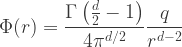
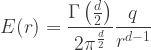
![\displaystyle{\begin{aligned} E(r) &= -\frac{d\Phi(r)}{dr} \\ \\ \int_r^{\infty} d\Phi &= - \frac{\Gamma\left( \frac{d}{2} \right)}{2 \pi^{\frac{d}{2}}} q \int_r^{\infty} r^{-d+1} dr \\ \\ \Phi(\infty) - \Phi(r) &= \frac{\Gamma\left( \frac{d}{2} \right)}{4 \pi^{\frac{d}{2}}} \frac{q}{\frac{d}{2}-1} \left[\frac{1}{r^{d-2}} \right]_r^{\infty} \\ \\ \Gamma (z) &= \frac{\Gamma (z+1)}{z} \\ \\ \Phi(r) &= \frac{\Gamma\left( \frac{d}{2} - 1\right)}{4 \pi^{\frac{d}{2}}} \frac{q}{r^{d-2}} \\ \\ \end{aligned} }](https://s0.wp.com/latex.php?latex=%5Cdisplaystyle%7B%5Cbegin%7Baligned%7D++++++++E%28r%29+%26%3D+-%5Cfrac%7Bd%5CPhi%28r%29%7D%7Bdr%7D++%5C%5C+%5C%5C++++%5Cint_r%5E%7B%5Cinfty%7D+d%5CPhi+%26%3D+-+%5Cfrac%7B%5CGamma%5Cleft%28+%5Cfrac%7Bd%7D%7B2%7D+%5Cright%29%7D%7B2+%5Cpi%5E%7B%5Cfrac%7Bd%7D%7B2%7D%7D%7D+q+%5Cint_r%5E%7B%5Cinfty%7D+r%5E%7B-d%2B1%7D+dr++%5C%5C+%5C%5C++++%5CPhi%28%5Cinfty%29+-+%5CPhi%28r%29+%26%3D+%5Cfrac%7B%5CGamma%5Cleft%28+%5Cfrac%7Bd%7D%7B2%7D+%5Cright%29%7D%7B4+%5Cpi%5E%7B%5Cfrac%7Bd%7D%7B2%7D%7D%7D+%5Cfrac%7Bq%7D%7B%5Cfrac%7Bd%7D%7B2%7D-1%7D+%5Cleft%5B%5Cfrac%7B1%7D%7Br%5E%7Bd-2%7D%7D+%5Cright%5D_r%5E%7B%5Cinfty%7D+++%5C%5C+%5C%5C++++%5CGamma+%28z%29+%26%3D+%5Cfrac%7B%5CGamma+%28z%2B1%29%7D%7Bz%7D+%5C%5C+%5C%5C+++++%5CPhi%28r%29+%26%3D+%5Cfrac%7B%5CGamma%5Cleft%28+%5Cfrac%7Bd%7D%7B2%7D+-+1%5Cright%29%7D%7B4+%5Cpi%5E%7B%5Cfrac%7Bd%7D%7B2%7D%7D%7D+%5Cfrac%7Bq%7D%7Br%5E%7Bd-2%7D%7D++++%5C%5C+%5C%5C+++++++++%5Cend%7Baligned%7D++%7D&bg=ffffff&fg=333333&s=1&c=20201002)
 implies that
  . Explain why this condition is satisfied by the ansatz
  .
.


 1 32
QPochhammer[-(-------), x]
Sqrt[x]
------------------------------------
1 32 8
(1 + -------) x QPochhammer[x, x]
Sqrt[x]
                     1        32
    QPochhammer[-(-------), x]
                  Sqrt[x]
------------------------------------
        1    32                    8
(1 + -------)   x QPochhammer[x, x]
     Sqrt[x]


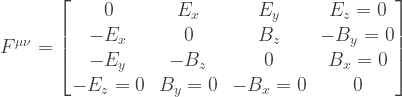
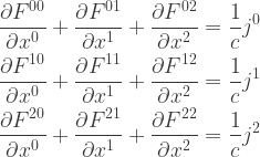
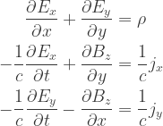
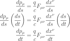
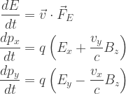
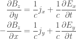
 , examine
  , the Maxwell equations (3.34), and the relativistic form of the force law derived in Problem 3.1.
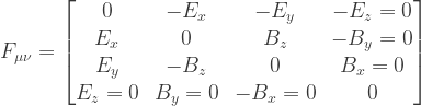


 direction.


You must be logged in to post a comment.