Consistent histories, origin

Posted on January 23, 2021 by rpflee

The square root of the probability, 6

There is no wave function collapse.

For example, in the double-slit experiment, with-detector and without-detector are actually two different physics systems. Different experimental setups provide different probability distributions, encoded in the wave functions. So different experimental setups result in different wave functions.

That is the key to understanding strange quantum phenomena such as EPR. A classical system has consistent results is no magic.

You create either a system with a detector or a system without a detector. With a detector, it will have only distinguishable-at-least-in-definition states, aka classical states. A system with only classical states is a classical system. Then, why so shocked when a classical system has consistent results?

Quantum mechanics is “strange”, but not “that strange”. It is not so strange that it is unexplainable.

— Me@2021-01-20 07:11 PM

— Me@2021-01-22 08:48 AM

Quantum Computing, 2.2

Posted on January 21, 2021 by rpflee

2021.01.21 Thursday ACHK

Summing over histories, 2

Posted on January 17, 2021 by rpflee

The square root of the probability, 5

If there is more than one way to achieve the present state, present == sum over all possible pasts, with weightings.

— Me@2011.06.26

This is false for a physical state. This is only true for wave functions, which are NOT probabilities.

Wave functions are used for calculating probabilities; but they are not themselves probabilities.

Wave functions are quantum states, but not physical states.

Wave functions are logical and mathematical, but not physical.

A physical state is something observable, something can be measured, at least in principle.

A physical state is something that exists in spacetime, a wave function is not.

— Me@2021-01-16 06:12:08 PM

The square root of the probability, 4.3

Posted on January 6, 2021 by rpflee

Eigenstates 3.4.3

The indistinguishability of cases is where the quantum probability comes from.

— Me@2020-12-25 06:21:48 PM

In the double slit experiment, there are 4 cases:

1. only the left slit is open

2. only the right slit is open

3. both slits are open and a measuring device is installed somewhere in the experiment setup so that we can know which slit each photon passes through

4. both slits are open but no measuring device is installed; so for each photon, we have no which-way information

For simplicity, we rephrase the case-3 and case-4:

1. only the left slit is open

2. only the right slit is open

3. both slits are open, with which-way information

4. both slits are open, without which-way information

Case-3 can be regarded as a classical overlapping of case-1 and case-2, because if you check the result of case-3, you will find that it is just an overlapping of result case-1 and result case-2.

However, case-4 cannot be regarded as a classical overlapping of case-1 and case-2. Instead, case-4 is a quantum superposition. A quantum superposition canNOT be regarded as a classical overlapping of possibilities/probabilities/worlds/universes.

Experimentally, no classical overlapping can explain the interference pattern, especially the destruction interference part. An addition of two non-zero probability values can never result in a zero.

Logically, case-4 is a quantum superposition of go-left and go-right. Case-4 is neither AND nor OR of the case-1 and case-2.

We can discuss AND or OR only when there are really 2 distinguishable cases. Since there are not any kinds of measuring devices (for getting which-way information) installed anywhere in the case-4, go-left and go-right are actually indistinguishable cases. In other words, by defining case-4 as a no-measuring-device case, we have indirectly defined that go-left and go-right are actually indistinguishable cases, even in principle.

Note that saying “they are actually indistinguishable cases, even in principle” is equivalent to saying that “they are logically indistinguishable cases” or “they are logically the same case“. So discussing whether a photon has gone left or gone right is meaningless.

If 2 cases are actually indistinguishable even in principle, then in a sense, there is actually only 1 case, the case of “both slits are open but without measuring device installed anywhere” (case-4). Mathematically, this case is expressed as the quantum superposition of go-left and go-right.

Since it is only 1 case, it is meaningless to discuss AND or OR. It is neither “go-left AND go-right” nor “go-left OR go-right“, because the phrases “go-left” and “go-right” are themselves meaningless in this case.

— Me@2020-12-19 10:38 AM

— Me@2020-12-26 11:02 AM

It is a quantum superposition of go-left and go-right.

Quantum superposition is NOT an overlapping of worlds.

Quantum superposition is neither AND nor OR.

— Me@2020-12-26 09:07:22 AM

When the final states are distinguishable you add probabilities:

$\displaystyle{P_{dis} = P_1 + P_2 = \psi_1^*\psi_1 + \psi_2^*\psi_2}$

.

When the final state are indistinguishable,[^2] you add amplitudes:

$\displaystyle{\Psi_{1,2} = \psi_1 + \psi_2}$

and

$\displaystyle{P_{ind} = \Psi_{1,2}^*\Psi_{1,2} = \psi_1^*\psi_1 + \psi_1^*\psi_2 + \psi_2^*\psi_1 + \psi_2^*\psi_2}$

.

[^2]: This is not precise, the states need to be “coherent”, but you don’t want to hear about that today.

edited Mar 21 ’13 at 17:04
answered Mar 21 ’13 at 16:58

dmckee

— Physics Stack Exchange

.

$\displaystyle{ P_{ind} = P_1 + P_2 + \psi_2^*\psi_1 + \psi_2^*\psi_2 }$

$\displaystyle{ P_{\text{indistinguishable}} = P_{\text{distinguishable}} + \text{interference terms} }$

— Me@2020-12-26 09:07:46 AM

interference terms ~ indistinguishability effect

— Me@2020-12-26 01:22:36 PM

The square root of the probability, 4.2

Posted on December 30, 2020 by rpflee

Eigenstates 3.4.2

The difference between quantum and classical is due to the indistinguishability of cases.

— Me@2020-12-26 01:25:03 PM

Statistical effects of indistinguishability

The indistinguishability of particles has a profound effect on their statistical properties.

The differences between the statistical behavior of fermions, bosons, and distinguishable particles can be illustrated using a system of two particles. The particles are designated A and B. Each particle can exist in two possible states, labelled $\displaystyle{ |0 \rangle }$ and $\displaystyle{|1\rangle}$ , which have the same energy.

The composite system can evolve in time, interacting with a noisy environment. Because the $\displaystyle{|0\rangle}$ and $\displaystyle{|1\rangle}$ states are energetically equivalent, neither state is favored, so this process has the effect of randomizing the states. (This is discussed in the article on quantum entanglement.) After some time, the composite system will have an equal probability of occupying each of the states available to it. The particle states are then measured.

If A and B are distinguishable particles, then the composite system has four distinct states: $\displaystyle{|0\rangle |0\rangle}$ , $\displaystyle{|1\rangle |1\rangle}$ , $\displaystyle{ |0\rangle |1\rangle}$ , and $\displaystyle{|1\rangle |0\rangle }$ . The probability of obtaining two particles in the $\displaystyle{|0\rangle}$ state is 0.25; the probability of obtaining two particles in the $\displaystyle{|1\rangle}$ state is 0.25; and the probability of obtaining one particle in the $\displaystyle{|0\rangle}$ state and the other in the $\displaystyle{|1\rangle}$ state is 0.5.

If A and B are identical bosons, then the composite system has only three distinct states: $\displaystyle{|0\rangle |0\rangle}$ , $\displaystyle{ |1\rangle |1\rangle }$ , and $\displaystyle{{\frac {1}{\sqrt {2}}}(|0\rangle |1\rangle +|1\rangle |0\rangle)}$ . When the experiment is performed, the probability of obtaining two particles in the $\displaystyle{|0\rangle}$ is now 0.33; the probability of obtaining two particles in the $\displaystyle{|1\rangle}$ state is 0.33; and the probability of obtaining one particle in the $\displaystyle{|0\rangle}$ state and the other in the $\displaystyle{|1\rangle}$ state is 0.33. Note that the probability of finding particles in the same state is relatively larger than in the distinguishable case. This demonstrates the tendency of bosons to “clump.”

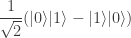
If A and B are identical fermions, there is only one state available to the composite system: the totally antisymmetric state $\displaystyle{{\frac {1}{\sqrt {2}}}(|0\rangle |1\rangle -|1\rangle |0\rangle)}$ . When the experiment is performed, one particle is always in the $\displaystyle{|0\rangle}$ state and the other is in the $\displaystyle{|1\rangle}$ state.

The results are summarized in Table 1:

— Wikipedia on Identical particles

The square root of the probability, 4

Posted on December 27, 2020 by rpflee

Eigenstates 3.4

quantum ~ classical with the indistinguishability of cases

— Me@2020-12-23 06:19:00 PM

In statistical mechanics, a semi-classical derivation of the entropy that does not take into account the indistinguishability of particles, yields an expression for the entropy which is not extensive (is not proportional to the amount of substance in question). This leads to a paradox known as the Gibbs paradox, after Josiah Willard Gibbs who proposed this thought experiment in 1874‒1875. The paradox allows for the entropy of closed systems to decrease, violating the second law of thermodynamics. A related paradox is the “mixing paradox”. If one takes the perspective that the definition of entropy must be changed so as to ignore particle permutation, the paradox is averted.

— Wikipedia on Gibbs paradox

Pointer state, 3

Posted on December 18, 2020 by rpflee

Eigenstates 3.3 | The square root of the probability, 3

In calculation, if a quantum state is in a superposition, that superposition is a superposition of eigenstates.

However, real superposition does not just include eigenstates that make macroscopic senses.

That is the major mistake of the many-worlds interpretation of quantum mechanics.

— Me@2017-12-30 10:24 AM

— Me@2018-07-03 07:24 PM

— Me@2020-12-18 06:12 PM

Mathematically, a quantum superposition is a superposition of eigenstates. An eigenstate is a quantum state that is corresponding to a macroscopic state. A superposition state is a quantum state that has no classical correspondence.

The macroscopic states are the only observable states. An observable state is one that can be measured directly or indirectly. For an unobservable state, we write it as a superposition of eigenstates. We always write a superposition state as a superposition of observable states; so in this sense, before measurement, we can almost say that the system is in a superposition of different (possible) classical macroscopic universes.

However, conceptually, especially when thinking in terms of Feynman’s summing over histories picture, a quantum state is more than a superposition of classical states. In other words, a system can have a quantum state which is a superposition of not only normal classical states, but also bizarre classical states and eigen-but-classically-impossible states.

A bizarre classical state is a state that follows classical physical laws, but is highly improbable that, in daily life language, we label such a state “impossible”, such as a human with five arms.

An eigen-but-classically-impossible state is a state that violates classical physical laws, such as a castle floating in the sky.

For a superposition, if we allow only normal classical states as the component eigenstates, a lot of the quantum phenomena, such as quantum tunnelling, cannot be explained.

If you want multiple universes, you have to include not only normal universes, but also the bizarre ones.

Actually, even for the double-slit experiment, “superposition of classical states” is not able to explain the existence of the interference patterns.

The superposition of the electron-go-left universe and the electron-go-right universe does not form this universe, where the interference patterns exist.

— Me@2020-12-16 05:18:03 PM

One of the reasons is that a quantum superposition is not a superposition of different possibilities/probabilities/worlds/universes, but a superposition of quantum eigenstates, which, in a sense, are square roots of probabilities.

— Me@2020-12-18 06:07:22 PM

The square root of the probability, 2

Posted on August 4, 2020 by rpflee

Mixed states, 4.2

Superposition in quantum mechanics is a complex number superposition.

— Me@2017-08-02 02:56:23 PM

Superposition in quantum mechanics is not a superposition of probabilities.

Instead, it is a superposition of probability amplitudes, which have complex number values.

Probability amplitude, in a sense, is the square root of probability.

— Me@2020-08-04 03:38:43 PM

Quantum entanglement, 4

Posted on July 20, 2020 by rpflee

What’s sneaky about quantum mechanics is that the whole system can be in a pure state which when restricted to each subsystem gives a mixed state, and that these mixed states are then correlated (necessarily, as it turns out). That’s what “entanglement” is all about.

…

The first way things get trickier in quantum mechanics is that something we are used to in classical mechanics fails. In classical mechanics, pure states are always dispersion-free — that is, for every observable, the probability measure assigned by the state to that observable is a Dirac delta measure, that is, the observable has a 100% chance of being some specific value and a 0% chance of having any other value. (Consider the example of the dice, with the observable being the number of dots on the face pointing up.) In quantum mechanics, pure states need NOT be dispersion-free. In fact, they usually aren’t.

A second, subtler way things get trickier in quantum mechanics concerns systems made of parts, or subsystems. Every observable of a subsystem is automatically an observable for the whole system (but not all observables of the whole system are of that form; some involve, say, adding observables of two different subsystems). So every state of the whole system gives rise to, or as we say, “restricts to,” a state of each of its subsystems. In classical mechanics, pure states restrict to pure states. For example, if our system consisted of 2 dice, a pure state of the whole system would be something like “the first die is in state 2 and the second one is in state 5;” this restricts to a pure state for the first die (state 2) and a pure state for the second die (state 5). In quantum mechanics, it is not true that a pure state of a system must restrict to a pure state of each subsystem.

It is this latter fact that gave rise to a whole bunch of quantum puzzles such as the Einstein-Podolsky-Rosen puzzle and Bell’s inequality. And it is this last fact that makes things a bit tricky when one of the two subsystems happens to be you. It is possible, and indeed very common, for the following thing to happen when two subsystems interact as time passes. Say the whole system starts out in a pure state which restricts to a pure state of each subsystem. After a while, this need no longer be the case! Namely, if we solve Schroedinger’s equation to calculate the state of the system a while later, it will necessarily still be a pure state (pure states of the whole system evolve to pure states), but it need no longer restrict to pure states of the two subsystems. If this happens, we say that the two subsystems have become “entangled.”

— December 16, 1993

— This Week’s Finds in Mathematical Physics (Week 27)

— John Baez

2020.07.19 Sunday ACHK

Frequency probability and Bayesian probability, 2.2

Posted on January 26, 2020 by rpflee

The probability frequentist vs Bayesian debate can be transcended by realizing that an observer cannot be separated from the observed.

— Me@2011.07.23

Quantum Computing, 3

Posted on August 24, 2019 by rpflee

Instead of requiring deterministic calculation, you allow (quantum) probabilistic calculation. What you gain is the extra speed.

— Me@2018-02-08 01:50:06 PM

Classical probability, 7

Posted on May 3, 2019 by rpflee

Classical probability is macroscopic superposition.

— Me@2012.04.23

That is not correct, except in some special senses.

— Me@2019-05-02

That is not correct, if the “superposition” means quantum superposition.

— Me@2019-05-03 08:44:11 PM

The difference of the classical probability and quantum probability is the difference of a mixed state and a pure superposition state.

In classical probability, the relationship between mutually exclusive possible measurement results, before measurement, is OR.

In quantum probability, if the quantum system is in quantum superposition, the relationship between mutually exclusive possible measurement results, before measurement, is neither OR nor AND.

— Me@2019-05-03 06:04:27 PM

Mixed states, 4

Posted on April 23, 2019 by rpflee

How is quantum superposition different from mixed state?

The state

$\displaystyle{|\Psi \rangle = \frac{1}{\sqrt{2}}\left(|\psi_1\rangle +|\psi_2\rangle \right)}$

is a pure state. Meaning, there’s not a 50% chance the system is in the state $\displaystyle{|\psi_1 \rangle }$ and a 50% it is in the state $\displaystyle{|\psi_2 \rangle}$ . There is a 0% chance that the system is in either of those states, and a 100% chance the system is in the state $\displaystyle{|\Psi \rangle}$ .

The point is that these statements are all made before I make any measurements.

— edited Jan 20 ’15 at 9:54

— Mehrdad

— answered Oct 12 ’13 at 1:42

— Andrew

Given a state, mixed or pure, you can compute the probability distribution $\displaystyle{P(\lambda_n)}$ for measuring eigenvalues $\displaystyle{\lambda_n}$ , for any observable you want. The difference is the way you combine probabilities, in a quantum superposition you have complex numbers that can interfere. In a classical probability distribution things only add positively.

— Andrew Oct 12 ’13 at 14:41

— How is quantum superposition different from mixed state?

— Physics StackExchange

2019.04.23 Tuesday ACHK

The problem of induction 3.3

Posted on December 28, 2018 by rpflee

“Everything has no patterns” (or “there are no laws”) creates a paradox.

If “there are 100% no first order laws”, then it is itself a second order law (the law of no first-order laws), allowing you to use probability theory.

In this sense, probability theory is a second order law: the law of “there are 100% no first order laws”.

In this sense, probability theory is not for a single event, but statistical, for a meta-event: a collection of events.

Using meta-event patterns to predict the next single event, that is induction.

Induction is a kind of risk minimization.

— Me@2012-11-05 12:23:24 PM

The problem of induction 3.1.2

Posted on December 18, 2018 by rpflee

Square of opposition

“everything has a pattern”?

“everything follows some pattern” –> no paradox

“everything follows no pattern” –> paradox

— Me@2012.11.05

My above statements are meaningless, because they lack a precise meaning of the word “pattern”. In other words, whether each statement is correct or not, depends on the meaning of “pattern”.

In common usage, “pattern” has two possible meanings:

1. “X has a pattern” can mean that “X has repeated data“.

Since the data set X has repeated data, we can simplify X’s description.

For example, there is a die. You throw it a thousand times. The result is always 2. Then you do not have to record a thousand 2’s. Instead, you can just record “the result is always 2”.

2. “X has a pattern” can mean that “X’s are totally random, in the sense that individual result cannot be precisely predicted“.

Since the data set X is totally random, we can simplify the description using probabilistic terms.

For example, there is a die. You throw it a thousand times. The die lands on any of the 6 faces 1/6 of the times. Then you do not have to record those thousand results. Instead, you can just record “the result is random” or “the die is fair”.

— Me@2018-12-18 12:34:58 PM

The problem of induction 3.2

Posted on December 10, 2018 by rpflee

The meaning of induction is that

we regard, for example, that

“AAAAA –> the sixth is also A”

is more likely than

“AA –> the second is also A”

We use induction to find “patterns”. However, the induced results might not be true. Then, why do we use induction at all?

There is everything to win but nothing to lose.

— Hans Reichenbach

If the universe has some patterns, we can use induction to find those patterns.

But if the universe has no patterns at all, then we cannot use any methods, induction or else, to find any patterns.

However, to find patterns, besides induction, what are the other methods?

What is meaning of “pattern-finding methods other than induction”?

— Me@2012.11.05

— Me@2018.12.10

Double slit experiment, 8

Posted on November 27, 2018 by rpflee

Although the screen itself is a photon position detector, it gets no which-way information. So it can get an interference pattern.

— Me@2012-04-09 7:24:23 PM

The problem of induction 3

Posted on November 20, 2018 by rpflee

In a sense (of the word “pattern”), there is always a pattern.

Where if there are no patterns, everything is random?

Then we have a meta-pattern; we can use probability laws:

In that case, every (microscopic) case is equally probable. Then by counting the possible number of microstates of each macrostate, we can deduce that which macrostate is the most probable.

Where if not all microstates are equally probable?

Then it has patterns directly.

For example, we can deduce that which microstate is the most probable.

— Me@2012.11.05

Monty Hall problem 1.6

Posted on November 2, 2018 by rpflee

Sasha Volokh (2015) wrote that “any explanation that says something like ‘the probability of door 1 was 1/3, and nothing can change that…’ is automatically fishy: probabilities are expressions of our ignorance about the world, and new information can change the extent of our ignorance.”

— Wikipedia on Monty Hall problem

2018.11.02 Friday ACHK

The square root of the probability

Posted on August 19, 2018 by rpflee

Probability amplitude in Layman’s Terms

What I understood is that probability amplitude is the square root of the probability … but the square root of the probability does not mean anything in the physical sense.

Can any please explain the physical significance of the probability amplitude in quantum mechanics?

edited Mar 1 at 16:31
nbro

asked Mar 21 ’13 at 15:36
Deepu

Part of you problem is

“Probability amplitude is the square root of the probability […]”

The amplitude is a complex number whose amplitude is the probability. That is $\psi^* \psi = P$ where the asterisk superscript means the complex conjugate. ${}^{[1]}$ It may seem a little pedantic to make this distinction because so far the “complex phase” of the amplitudes has no effect on the observables at all: we could always rotate any given amplitude onto the positive real line and then “the square root” would be fine.

But we can’t guarantee to be able to rotate more than one amplitude that way at the same time.

More over, there are two ways to combine amplitudes to find probabilities for observation of combined events.

When the final states are distinguishable you add probabilities:

$P_{dis} = P_1 + P_2 = \psi_1^* \psi_1 + \psi_2^* \psi_2$

When the final state are indistinguishable, ${}^{[2]}$ you add amplitudes:

$\Psi_{1,2} = \psi_1 + \psi_2$

and

$P_{ind} = \Psi_{1,2}^*\Psi_{1,2} = \psi_1^*\psi_1 + \psi_1^*\psi_2 + \psi_2^*\psi_1 + \psi_2^* \psi_2$

The terms that mix the amplitudes labeled 1 and 2 are the “interference terms”. The interference terms are why we can’t ignore the complex nature of the amplitudes and they cause many kinds of quantum weirdness.

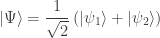
${}^1$ Here I’m using a notation reminiscent of a Schrödinger-like formulation, but that interpretation is not required. Just accept $\psi$ as a complex number representing the amplitude for some observation.

${}^2$ This is not precise, the states need to be “coherent”, but you don’t want to hear about that today.

edited Mar 21 ’13 at 17:04
answered Mar 21 ’13 at 16:58

dmckee

— Physics Stack Exchange

Physics Town

continues

Category Archives: quantum probability

Consistent histories, origin

Quantum Computing, 2.2

Summing over histories, 2

The square root of the probability, 4.3

The square root of the probability, 4.2

The square root of the probability, 4

Pointer state, 3

The square root of the probability, 2

Quantum entanglement, 4

Frequency probability and Bayesian probability, 2.2

Quantum Computing, 3

Classical probability, 7

Mixed states, 4

The problem of induction 3.3

The problem of induction 3.1.2

The problem of induction 3.2

Double slit experiment, 8

The problem of induction 3

Monty Hall problem 1.6

The square root of the probability