Ex 1.24 Constraint forces, 1.1
Structure and Interpretation of Classical Mechanics
.
~~~
[guess]


.


.
(define (KE-particle m v)
  (* 1/2 m (square v)))

(define ((extract-particle pieces) local i)
  (let* ((indices (apply up (iota pieces (* i pieces))))
         (extract (lambda (tuple)
                    (vector-map (lambda (i)
                                  (ref tuple i))
                                indices))))
    (up (time local)
        (extract (coordinate local))
        (extract (velocity local)))))

(define (U-constraint q0 q1 F l)
  (* (/ F (* 2 l))
     (- (square (- q1 q0))
        (square l))))

(define ((U-gravity g m) q)
  (let* ((y (ref q 1)))
    (* m g y)))

(define ((L-driven-free m l x_s y_s U) local)
  (let* ((extract (extract-particle 2))

     (p (extract local 0))
     (q (coordinate p))
     (qdot (velocity p))

     (F (ref (coordinate local) 2)))

    (- (KE-particle m qdot)
       (U q)
       (U-constraint (up (x_s (time local)) (y_s (time local)))
             q
             F
             l))))

(let* ((U (U-gravity 'g 'm))
       (x_s (literal-function 'x_s))
       (y_s (literal-function 'y_s))
       (L (L-driven-free 'm 'l x_s y_s U))
       (q-rect (up (literal-function 'x)
                   (literal-function 'y)
                   (literal-function 'F))))
  (show-expression
   ((compose L (Gamma q-rect)) 't)))
![\displaystyle{ L = \frac{1}{2} m \left[(Dx)^2 + (Dy)^2 \right] - mgy - \frac{F}{2l} \left[ (x-x_s)^2 + (y-y_s)^2 - l^2 \right] }](https://s0.wp.com/latex.php?latex=%5Cdisplaystyle%7B+L+%3D+%5Cfrac%7B1%7D%7B2%7D+m+%5Cleft%5B%28Dx%29%5E2+%2B+%28Dy%29%5E2+%5Cright%5D+-+mgy+-+%5Cfrac%7BF%7D%7B2l%7D+%5Cleft%5B+%28x-x_s%29%5E2+%2B+%28y-y_s%29%5E2+-+l%5E2+%5Cright%5D+%7D&bg=ffffff&fg=333333&s=0&c=20201002)
(let* ((U (U-gravity 'g 'm))
       (x_s (literal-function 'x_s))
       (y_s (literal-function 'y_s))
       (L (L-driven-free 'm 'l x_s y_s U))
       (q-rect (up (literal-function 'x)
                   (literal-function 'y)
                   (literal-function 'F))))
  (show-expression
   (((Lagrange-equations L) q-rect) 't)))
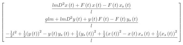
![\displaystyle{ \begin{aligned} mD^2x(t) + \frac{F(t)}{l} \left[x(t) - x_s(t)\right] &= 0 \\ mg + m D^2y(t) + \frac{F(t)}{l} [y(t) - y_s(t)] &= 0 \\ -l^2 + [y(t)-y_s(t)]^2 + [x(t)-x_s(t)]^2 &= 0 \\ \end{aligned}}](https://s0.wp.com/latex.php?latex=%5Cdisplaystyle%7B+%5Cbegin%7Baligned%7D+mD%5E2x%28t%29+%2B+%5Cfrac%7BF%28t%29%7D%7Bl%7D+%5Cleft%5Bx%28t%29+-+x_s%28t%29%5Cright%5D+%26%3D+0+%5C%5C+mg+%2B+m+D%5E2y%28t%29+%2B+%5Cfrac%7BF%28t%29%7D%7Bl%7D+%5By%28t%29+-+y_s%28t%29%5D+%26%3D+0+%5C%5C+-l%5E2+%2B+%5By%28t%29-y_s%28t%29%5D%5E2+%2B+%5Bx%28t%29-x_s%28t%29%5D%5E2+%26%3D+0+%5C%5C+%5Cend%7Baligned%7D%7D&bg=ffffff&fg=333333&s=0&c=20201002)
(define ((F->C F) local)
(->local (time local)
(F local)
(+ (((partial 0) F) local)
(* (((partial 1) F) local)
(velocity local)))))
(define ((q->r x_s y_s l) local)
(let* ((q (coordinate local))
(t (time local))
(theta (ref q 0))
(F (ref q 1)))
(up (+ (x_s t) (* l (sin theta)))
(- (y_s t) (* l (cos theta)))
F)))
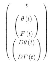
(let ((q (up (literal-function 'theta)
(literal-function 'F))))
(show-expression (q 't)))

(let* ((x_s (literal-function 'x_s))
       (y_s (literal-function 'y_s))
       (q (up (literal-function 'theta)
              (literal-function 'F))))
  (show-expression ((Gamma q) 't)))
(let* ((xs (literal-function 'x_s))
(ys (literal-function 'y_s))
(q (up (literal-function 'theta)
(literal-function 'F))))
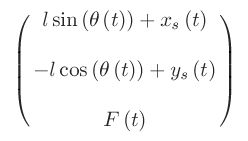
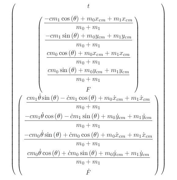
(show-expression ((compose (q->r xs ys 'l) (Gamma q)) 't)))
(let* ((xs (literal-function 'x_s))
       (ys (literal-function 'y_s))
       (q (up (literal-function 'theta)
              (literal-function 'F))))
  (show-expression ((F->C (q->r xs ys 'l)) ((Gamma q) 't))))

(define (L-theta m l x_s y_s U)
  (compose
   (L-driven-free m l x_s y_s U) (F->C (q->r x_s y_s l))))

(let* ((U (U-gravity 'g 'm))
       (xs (literal-function 'x_s))
       (ys (literal-function 'y_s))
       (q (up (literal-function 'theta)
              (literal-function 'F))))
  (show-expression ((Gamma
                    (compose (q->r xs ys 'l) (Gamma q)))
                    't)))

(let* ((U (U-gravity 'g 'm))
       (xs (literal-function 'x_s))
       (ys (literal-function 'y_s))
       (q (up (literal-function 'theta)
              (literal-function 'F))))
  (show-expression (U ((compose (q->r xs ys 'l) (Gamma q)) 't))))
(let* ((U (U-gravity 'g 'm))
       (xs (literal-function 'x_s))
       (ys (literal-function 'y_s))
       (q (up (literal-function 'theta)
              (literal-function 'F))))
  (show-expression ((L-driven-free 'm 'l xs ys U)
		    ((Gamma (compose (q->r xs ys 'l) (Gamma q))) 't))))

(let* ((U (U-gravity 'g 'm))
(xs (literal-function 'x_s))
(ys (literal-function 'y_s))
(q (up (literal-function 'theta)
(literal-function 'F))))
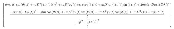
(show-expression ((L-theta 'm 'l xs ys U) ((Gamma q) 't))))
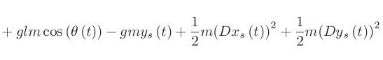
![\displaystyle{ \begin{aligned} L_\theta &= \frac{1}{2} m (D x_s(t))^2 + \frac{1}{2} m (D y_s(t))^2 - m g \left[ y_s(t) - l \cos \theta(t) \right] \\ &+ \frac{1}{2} m l^2 (D \theta(t))^2 + lm D \theta(t) \left[ D x_s(t) \cos \theta(t) + \sin \theta(t) D y_s(t) \right] \\ \end{aligned}}](https://s0.wp.com/latex.php?latex=%5Cdisplaystyle%7B+%5Cbegin%7Baligned%7D+++L_%5Ctheta+++++%26%3D+++%5Cfrac%7B1%7D%7B2%7D+m+%28D+x_s%28t%29%29%5E2++%2B+%5Cfrac%7B1%7D%7B2%7D+m+%28D+y_s%28t%29%29%5E2++-++m+g+%5Cleft%5B+y_s%28t%29+-+l+%5Ccos+%5Ctheta%28t%29++%5Cright%5D+%5C%5C++%26%2B+%5Cfrac%7B1%7D%7B2%7D+m+l%5E2+%28D+%5Ctheta%28t%29%29%5E2+++%2B+lm+D+%5Ctheta%28t%29+%5Cleft%5B+++++D+x_s%28t%29+%5Ccos+%5Ctheta%28t%29+%2B+%5Csin+%5Ctheta%28t%29+D+y_s%28t%29++%5Cright%5D++++%5C%5C+++%5Cend%7Baligned%7D%7D&bg=ffffff&fg=333333&s=0&c=20201002)
[guess]
— Me@2022-03-24 04:38:10 PM
.
.
2022.03.26 Saturday (c) All rights reserved by ACHK


![\displaystyle{ D(F \circ \Gamma[q]) = (DF\circ\Gamma[q])D\Gamma[q] }](https://s0.wp.com/latex.php?latex=%5Cdisplaystyle%7B++D%28F+%5Ccirc+%5CGamma%5Bq%5D%29+%3D+%28DF%5Ccirc%5CGamma%5Bq%5D%29D%5CGamma%5Bq%5D+++%7D&bg=ffffff&fg=333333&s=0&c=20201002)
![\displaystyle{ DF \circ \Gamma[q] = \left[ \partial_0 F \circ \Gamma[q], \partial_1 F \circ \Gamma[q], \partial_2 F \circ \Gamma[q], ... \right] }](https://s0.wp.com/latex.php?latex=%5Cdisplaystyle%7B++DF+%5Ccirc+%5CGamma%5Bq%5D+%3D+%5Cleft%5B+%5Cpartial_0+F+%5Ccirc+%5CGamma%5Bq%5D%2C+%5Cpartial_1+F+%5Ccirc+%5CGamma%5Bq%5D%2C+%5Cpartial_2+F+%5Ccirc+%5CGamma%5Bq%5D%2C+...++%5Cright%5D+++%7D&bg=ffffff&fg=333333&s=0&c=20201002)
![\displaystyle{ \left(D \Gamma[q] \right)(t) = \left( 1, Dq(t), D^2 q(t), ... \right) = \begin{bmatrix} 1 \\ Dq(t) \\ D^2 q(t) \\ ... \\ \end{bmatrix} \\ }](https://s0.wp.com/latex.php?latex=%5Cdisplaystyle%7B++%5Cleft%28D+%5CGamma%5Bq%5D+%5Cright%29%28t%29+++%3D+%5Cleft%28+1%2C+Dq%28t%29%2C+D%5E2+q%28t%29%2C+...+%5Cright%29++%3D+%5Cbegin%7Bbmatrix%7D+1+%5C%5C+Dq%28t%29+%5C%5C+D%5E2+q%28t%29+%5C%5C+...+%5C%5C+%5Cend%7Bbmatrix%7D+%5C%5C+++%7D&bg=ffffff&fg=333333&s=0&c=20201002)
![\displaystyle{ \begin{aligned} D(F \circ \Gamma[q])(t) &= (DF\circ\Gamma[q])D\Gamma[q](t) \\ &= \left[ \partial_0 F \circ \Gamma[q], \partial_1 F \circ \Gamma[q], \partial_2 F \circ \Gamma[q], ... \right] \begin{bmatrix} 1 \\ Dq(t) \\ D^2 q(t) \\ ... \\ \end{bmatrix} \\ &= \partial_0 F \circ \Gamma[q] + \partial_1 F \circ \Gamma[q] D q(t) + \partial_2 F \circ \Gamma[q] D^2 q(t) + ... \\ &= \partial_0 F \circ \Gamma[q] u(t) + \partial_1 F \circ \Gamma[q] D q(t) + \partial_2 F \circ \Gamma[q] D^2 q(t) + ... \\ \end{aligned} }](https://s0.wp.com/latex.php?latex=%5Cdisplaystyle%7B++%5Cbegin%7Baligned%7D++D%28F+%5Ccirc+%5CGamma%5Bq%5D%29%28t%29+++%26%3D+%28DF%5Ccirc%5CGamma%5Bq%5D%29D%5CGamma%5Bq%5D%28t%29+%5C%5C+++%26%3D+%5Cleft%5B+%5Cpartial_0+F+%5Ccirc+%5CGamma%5Bq%5D%2C+%5Cpartial_1+F+%5Ccirc+%5CGamma%5Bq%5D%2C+%5Cpartial_2+F+%5Ccirc+%5CGamma%5Bq%5D%2C+...++%5Cright%5D++++%5Cbegin%7Bbmatrix%7D+1+%5C%5C+Dq%28t%29+%5C%5C+D%5E2+q%28t%29+%5C%5C+...+%5C%5C+%5Cend%7Bbmatrix%7D+++%5C%5C+++%26%3D+%5Cpartial_0+F+%5Ccirc+%5CGamma%5Bq%5D+%2B+%5Cpartial_1+F+%5Ccirc+%5CGamma%5Bq%5D+D+q%28t%29+%2B+%5Cpartial_2+F+%5Ccirc+%5CGamma%5Bq%5D+D%5E2+q%28t%29+%2B+...+++%5C%5C+++%26%3D+%5Cpartial_0+F+%5Ccirc+%5CGamma%5Bq%5D+u%28t%29+%2B+%5Cpartial_1+F+%5Ccirc+%5CGamma%5Bq%5D+D+q%28t%29+%2B+%5Cpartial_2+F+%5Ccirc+%5CGamma%5Bq%5D+D%5E2+q%28t%29+%2B+...+++%5C%5C+++%5Cend%7Baligned%7D++%7D&bg=ffffff&fg=333333&s=0&c=20201002)

![\displaystyle{ \begin{aligned} D(F \circ \Gamma[q]) &= \partial_0 F \circ \Gamma[q] u + \partial_1 F \circ \Gamma[q] D q + \partial_2 F \circ \Gamma[q] D^2 q + ... \\ &= \partial_0 F \circ \Gamma[q] J_0 \circ \Gamma[q] + \partial_1 F \circ \Gamma[q] J_1 \circ \Gamma[q] + \partial_2 F \circ \Gamma[q] J_2 \circ \Gamma[q] + ... \\ \end{aligned} }](https://s0.wp.com/latex.php?latex=%5Cdisplaystyle%7B++%5Cbegin%7Baligned%7D++D%28F+%5Ccirc+%5CGamma%5Bq%5D%29++%26%3D+%5Cpartial_0+F+%5Ccirc+%5CGamma%5Bq%5D+u+%2B+%5Cpartial_1+F+%5Ccirc+%5CGamma%5Bq%5D+D+q+%2B+%5Cpartial_2+F+%5Ccirc+%5CGamma%5Bq%5D+D%5E2+q+%2B+...++++%5C%5C+++%26%3D+%5Cpartial_0+F+%5Ccirc+%5CGamma%5Bq%5D+J_0+%5Ccirc+%5CGamma%5Bq%5D+%2B+%5Cpartial_1+F+%5Ccirc+%5CGamma%5Bq%5D+J_1+%5Ccirc+%5CGamma%5Bq%5D+%2B+%5Cpartial_2+F+%5Ccirc+%5CGamma%5Bq%5D+J_2+%5Ccirc+%5CGamma%5Bq%5D+%2B+...++%5C%5C+++%5Cend%7Baligned%7D++%7D&bg=ffffff&fg=333333&s=0&c=20201002)
![\displaystyle{ \begin{aligned} I_0 \circ \Gamma[q] &= t \\ \\ I_{n>0} \circ \Gamma[q] &= I_{n>0} (t, q, v, a, ...) \\ &= I_{n>0} (t, q, Dq, D^2 q, ...) \\ &= D^{(n-1)} q \\ \\ J_{n} \circ \Gamma[q] &= D(I_n (t, q, v, a, ...)) \\ \end{aligned} }](https://s0.wp.com/latex.php?latex=%5Cdisplaystyle%7B++%5Cbegin%7Baligned%7D++I_0+%5Ccirc+%5CGamma%5Bq%5D+%26%3D+t+%5C%5C+%5C%5C++I_%7Bn%3E0%7D+%5Ccirc+%5CGamma%5Bq%5D+++%26%3D+I_%7Bn%3E0%7D+%28t%2C+q%2C+v%2C+a%2C+...%29+%5C%5C+++%26%3D+I_%7Bn%3E0%7D+%28t%2C+q%2C+Dq%2C+D%5E2+q%2C+...%29+%5C%5C+++%26%3D+D%5E%7B%28n-1%29%7D+q+%5C%5C+++++%5C%5C++J_%7Bn%7D+%5Ccirc+%5CGamma%5Bq%5D+++%26%3D+D%28I_n+%28t%2C+q%2C+v%2C+a%2C+...%29%29+%5C%5C+++%5Cend%7Baligned%7D++%7D&bg=ffffff&fg=333333&s=0&c=20201002)
is
![\displaystyle{\delta_\eta (f[q]g[q])}](https://s0.wp.com/latex.php?latex=%5Cdisplaystyle%7B%5Cdelta_%5Ceta+%28f%5Bq%5Dg%5Bq%5D%29%7D&bg=ffffff&fg=333333&s=0&c=20201002)
![\displaystyle{ \begin{aligned} D(F \circ \Gamma[q]) &= \partial_0 F \circ \Gamma[q] J_0 \circ \Gamma[q] + \partial_1 F \circ \Gamma[q] J_1 \circ \Gamma[q] + \partial_2 F \circ \Gamma[q] J_2 \circ \Gamma[q] + ... \\ &= \left[(\partial_0 F) J_0 + (\partial_1 F) J_1 + (\partial_2 F) J_2 + ... \right] \circ \Gamma[q] \\ \end{aligned} }](https://s0.wp.com/latex.php?latex=%5Cdisplaystyle%7B++%5Cbegin%7Baligned%7D++D%28F+%5Ccirc+%5CGamma%5Bq%5D%29++%26%3D+%5Cpartial_0+F+%5Ccirc+%5CGamma%5Bq%5D+J_0+%5Ccirc+%5CGamma%5Bq%5D+%2B+%5Cpartial_1+F+%5Ccirc+%5CGamma%5Bq%5D+J_1+%5Ccirc+%5CGamma%5Bq%5D+%2B+%5Cpartial_2+F+%5Ccirc+%5CGamma%5Bq%5D+J_2+%5Ccirc+%5CGamma%5Bq%5D+%2B+...++%5C%5C+++%26%3D+%5Cleft%5B%28%5Cpartial_0+F%29+J_0+%2B+%28%5Cpartial_1+F%29+J_1+%2B+%28%5Cpartial_2+F%29+J_2+%2B+...+%5Cright%5D+%5Ccirc+%5CGamma%5Bq%5D+++%5C%5C+++%5Cend%7Baligned%7D++%7D&bg=ffffff&fg=333333&s=0&c=20201002)
![\displaystyle{ D_t F \circ \Gamma[q] = D(F \circ \Gamma[q]) }](https://s0.wp.com/latex.php?latex=%5Cdisplaystyle%7B++D_t+F+%5Ccirc+%5CGamma%5Bq%5D+%3D+D%28F+%5Ccirc+%5CGamma%5Bq%5D%29++%7D&bg=ffffff&fg=333333&s=0&c=20201002)
![\displaystyle{ \begin{aligned} D_t F \circ \Gamma[q] &= \left[(\partial_0 F) J_0 + (\partial_1 F) J_1 + (\partial_2 F) J_2 + ... \right] \circ \Gamma[q] \\ \\ D_t F &= (\partial_0 F) J_0 + (\partial_1 F) J_1 + (\partial_2 F) J_2 + ... \\ \end{aligned} }](https://s0.wp.com/latex.php?latex=%5Cdisplaystyle%7B++%5Cbegin%7Baligned%7D++D_t+F+%5Ccirc+%5CGamma%5Bq%5D+++%26%3D+%5Cleft%5B%28%5Cpartial_0+F%29+J_0+%2B+%28%5Cpartial_1+F%29+J_1+%2B+%28%5Cpartial_2+F%29+J_2+%2B+...+%5Cright%5D+%5Ccirc+%5CGamma%5Bq%5D+++%5C%5C+%5C%5C++D_t+F+++%26%3D+%28%5Cpartial_0+F%29+J_0+%2B+%28%5Cpartial_1+F%29+J_1+%2B+%28%5Cpartial_2+F%29+J_2+%2B+...++++%5C%5C+++%5Cend%7Baligned%7D++%7D&bg=ffffff&fg=333333&s=0&c=20201002)

![\displaystyle{ \begin{aligned} D_t F \circ \Gamma[q] (t) &= \partial_0 F(t, q, v, a, ...) + \partial_1 F(t, q, v, a, ...) v(t) + \partial_2 F(t, q, v, a, ...) a(t) + ... \\ \end{aligned} }](https://s0.wp.com/latex.php?latex=%5Cdisplaystyle%7B++%5Cbegin%7Baligned%7D++D_t+F+%5Ccirc+%5CGamma%5Bq%5D+%28t%29++%26%3D+%5Cpartial_0+F%28t%2C+q%2C+v%2C+a%2C+...%29+%2B+%5Cpartial_1+F%28t%2C+q%2C+v%2C+a%2C+...%29+v%28t%29+%2B+%5Cpartial_2+F%28t%2C+q%2C+v%2C+a%2C+...%29+a%28t%29+%2B+...+++%5C%5C+++%5Cend%7Baligned%7D++%7D&bg=ffffff&fg=333333&s=0&c=20201002)
![\displaystyle{ \begin{aligned} &D_t (F + G) \circ \Gamma[q] (t) \\ \end{aligned} }](https://s0.wp.com/latex.php?latex=%5Cdisplaystyle%7B++%5Cbegin%7Baligned%7D++%26D_t+%28F+%2B+G%29+%5Ccirc+%5CGamma%5Bq%5D+%28t%29+%5C%5C++%5Cend%7Baligned%7D++%7D&bg=ffffff&fg=333333&s=0&c=20201002)
![\displaystyle{ \begin{aligned} &= \partial_0 \left[F(t, q, v, a, ...) + G(t, q, v, a, ...)\right] \\ &+ \partial_1 \left[F(t, q, v, a, ...) + G(t, q, v, a, ...)\right] v(t) \\ &+ \partial_2 \left[F(t, q, v, a, ...) + G(t, q, v, a, ...)\right] a(t) + ... \\ \end{aligned} }](https://s0.wp.com/latex.php?latex=%5Cdisplaystyle%7B++%5Cbegin%7Baligned%7D++%26%3D+%5Cpartial_0+%5Cleft%5BF%28t%2C+q%2C+v%2C+a%2C+...%29+%2B+G%28t%2C+q%2C+v%2C+a%2C+...%29%5Cright%5D+%5C%5C++++%26%2B+%5Cpartial_1+%5Cleft%5BF%28t%2C+q%2C+v%2C+a%2C+...%29+%2B+G%28t%2C+q%2C+v%2C+a%2C+...%29%5Cright%5D+v%28t%29+%5C%5C++++%26%2B+%5Cpartial_2+%5Cleft%5BF%28t%2C+q%2C+v%2C+a%2C+...%29+%2B+G%28t%2C+q%2C+v%2C+a%2C+...%29%5Cright%5D+a%28t%29+%2B+...+%5C%5C+++%5Cend%7Baligned%7D++%7D&bg=ffffff&fg=333333&s=0&c=20201002)
![\displaystyle{ \begin{aligned} &= \left[ \partial_0 F(t, q, v, a, ...) + \partial_0 G(t, q, v, a, ...)\right] \\ &+ \left[ \partial_1 F(t, q, v, a, ...) + \partial_1 G(t, q, v, a, ...)\right] v(t) \\ &+ \left[ \partial_2 F(t, q, v, a, ...) + \partial_2 G(t, q, v, a, ...)\right] a(t) + ... \\ \end{aligned} }](https://s0.wp.com/latex.php?latex=%5Cdisplaystyle%7B++%5Cbegin%7Baligned%7D++%26%3D+%5Cleft%5B+%5Cpartial_0+F%28t%2C+q%2C+v%2C+a%2C+...%29+%2B+%5Cpartial_0+G%28t%2C+q%2C+v%2C+a%2C+...%29%5Cright%5D+%5C%5C++++%26%2B+%5Cleft%5B+%5Cpartial_1+F%28t%2C+q%2C+v%2C+a%2C+...%29+%2B+%5Cpartial_1+G%28t%2C+q%2C+v%2C+a%2C+...%29%5Cright%5D+v%28t%29+%5C%5C++++%26%2B+%5Cleft%5B+%5Cpartial_2+F%28t%2C+q%2C+v%2C+a%2C+...%29+%2B+%5Cpartial_2+G%28t%2C+q%2C+v%2C+a%2C+...%29%5Cright%5D+a%28t%29+%2B+...+%5C%5C+++%5Cend%7Baligned%7D++%7D&bg=ffffff&fg=333333&s=0&c=20201002)

![\displaystyle{ \begin{aligned} &= D_t F \circ \Gamma[q] (t) + D_t G \circ \Gamma[q] (t) \\ \end{aligned} }](https://s0.wp.com/latex.php?latex=%5Cdisplaystyle%7B++%5Cbegin%7Baligned%7D++%26%3D+D_t+F+%5Ccirc+%5CGamma%5Bq%5D+%28t%29+%2B+D_t+G+%5Ccirc+%5CGamma%5Bq%5D+%28t%29+%5C%5C++%5Cend%7Baligned%7D++%7D&bg=ffffff&fg=333333&s=0&c=20201002)
![\displaystyle{ \begin{aligned} D_t (F + G) \circ \Gamma[q] (t) &= D_t F \circ \Gamma[q] (t) + D_t G \circ \Gamma[q] (t) \\ \end{aligned} }](https://s0.wp.com/latex.php?latex=%5Cdisplaystyle%7B++%5Cbegin%7Baligned%7D++D_t+%28F+%2B+G%29+%5Ccirc+%5CGamma%5Bq%5D+%28t%29+++%26%3D+D_t+F+%5Ccirc+%5CGamma%5Bq%5D+%28t%29+%2B+D_t+G+%5Ccirc+%5CGamma%5Bq%5D+%28t%29+%5C%5C+++%5Cend%7Baligned%7D++%7D&bg=ffffff&fg=333333&s=0&c=20201002)
![\displaystyle{ \begin{aligned} D_t (F + G) \circ \Gamma[q] (t) &= (D_t F + D_t G) \circ \Gamma[q] (t) \\ \\ D_t (F + G) \circ \Gamma[q] &= (D_t F + D_t G) \circ \Gamma[q] \\ \\ D_t (F + G) &= D_t F + D_t G \\ \end{aligned} }](https://s0.wp.com/latex.php?latex=%5Cdisplaystyle%7B++%5Cbegin%7Baligned%7D++D_t+%28F+%2B+G%29+%5Ccirc+%5CGamma%5Bq%5D+%28t%29+++%26%3D+%28D_t+F+%2B+D_t+G%29+%5Ccirc+%5CGamma%5Bq%5D+%28t%29+%5C%5C+++%5C%5C+++++++++D_t+%28F+%2B+G%29+%5Ccirc+%5CGamma%5Bq%5D++++%26%3D+%28D_t+F+%2B+D_t+G%29+%5Ccirc+%5CGamma%5Bq%5D++%5C%5C+++%5C%5C+++++++++D_t+%28F+%2B+G%29+++++%26%3D+D_t+F+%2B+D_t+G+++%5C%5C+++%5Cend%7Baligned%7D++%7D&bg=ffffff&fg=333333&s=0&c=20201002)


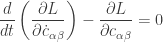
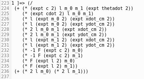
![\displaystyle{F(t) = l m \left[D \theta(t)\right]^2 + g m \cos \theta(t)}](https://s0.wp.com/latex.php?latex=%5Cdisplaystyle%7BF%28t%29+%3D+l+m+%5Cleft%5BD+%5Ctheta%28t%29%5Cright%5D%5E2+%2B+g+m+%5Ccos+%5Ctheta%28t%29%7D&bg=ffffff&fg=333333&s=0&c=20201002)
 ,
,  .
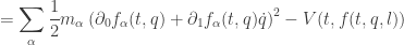
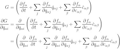
.![\displaystyle{ \begin{aligned} D ( \partial_2 L \circ \Gamma[q]) - (\partial_1 L \circ \Gamma[q]) &= 0 \\ \end{aligned}}](https://s0.wp.com/latex.php?latex=%5Cdisplaystyle%7B+%5Cbegin%7Baligned%7D+D+%28+%5Cpartial_2+L+%5Ccirc+%5CGamma%5Bq%5D%29+-+%28%5Cpartial_1+L+%5Ccirc+%5CGamma%5Bq%5D%29+%26%3D+0+%5C%5C+%5Cend%7Baligned%7D%7D&bg=ffffff&fg=333333&s=0&c=20201002)


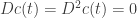
![\displaystyle{ - V(t, f(t,q,c)) - \sum_{\{ \alpha, \beta | \alpha < \beta, \alpha \leftrightarrow \beta \}} \frac{F_{\alpha \beta}}{2 l_{\alpha \beta}} \left[ c_{\alpha \beta}^2 - l_{\alpha \beta}^2 \right] }](https://s0.wp.com/latex.php?latex=%5Cdisplaystyle%7B+-+V%28t%2C+f%28t%2Cq%2Cc%29%29+-+%5Csum_%7B%5C%7B+%5Calpha%2C+%5Cbeta+%7C+%5Calpha+%3C+%5Cbeta%2C+%5Calpha+%5Cleftrightarrow+%5Cbeta+%5C%7D%7D+%5Cfrac%7BF_%7B%5Calpha+%5Cbeta%7D%7D%7B2+l_%7B%5Calpha+%5Cbeta%7D%7D+%5Cleft%5B+c_%7B%5Calpha+%5Cbeta%7D%5E2+-+l_%7B%5Calpha+%5Cbeta%7D%5E2+%5Cright%5D+%7D&bg=ffffff&fg=333333&s=0&c=20201002)

![\displaystyle{ \begin{aligned} &= \sum_\alpha \frac{1}{2} m_\alpha \left( \partial_0 f_\alpha (t;\{q_{\alpha i}\}, \{c_{\alpha \beta}\}) + \partial_1 f_\alpha (t;\{q_{\alpha i}\}, \{c_{\alpha \beta}\}) \dot q + \partial_2 f_\alpha (t;\{q_{\alpha i}\}, \{c_{\alpha \beta}\}) \dot c \right)^2 \\ &- V(t, f(t;\{q_{\alpha i}\}, \{c_{\alpha \beta}\})) - \sum_{\{ \alpha, \beta | \alpha < \beta, \alpha \leftrightarrow \beta \}} \frac{F_{\alpha \beta}}{2 l_{\alpha \beta}} \left[ c_{\alpha \beta}^2 - l_{\alpha \beta}^2 \right] \\ \end{aligned}}](https://s0.wp.com/latex.php?latex=%5Cdisplaystyle%7B+%5Cbegin%7Baligned%7D+++++%26%3D+%5Csum_%5Calpha+%5Cfrac%7B1%7D%7B2%7D+m_%5Calpha+%5Cleft%28+%5Cpartial_0+f_%5Calpha+%28t%3B%5C%7Bq_%7B%5Calpha+i%7D%5C%7D%2C+%5C%7Bc_%7B%5Calpha+%5Cbeta%7D%5C%7D%29+%2B+%5Cpartial_1+f_%5Calpha+%28t%3B%5C%7Bq_%7B%5Calpha+i%7D%5C%7D%2C+%5C%7Bc_%7B%5Calpha+%5Cbeta%7D%5C%7D%29+%5Cdot+q+%2B+%5Cpartial_2+f_%5Calpha+%28t%3B%5C%7Bq_%7B%5Calpha+i%7D%5C%7D%2C+%5C%7Bc_%7B%5Calpha+%5Cbeta%7D%5C%7D%29+%5Cdot+c+%5Cright%29%5E2+%5C%5C+++++%26-+V%28t%2C+f%28t%3B%5C%7Bq_%7B%5Calpha+i%7D%5C%7D%2C+%5C%7Bc_%7B%5Calpha+%5Cbeta%7D%5C%7D%29%29+-+%5Csum_%7B%5C%7B+%5Calpha%2C+%5Cbeta+%7C+%5Calpha+%3C+%5Cbeta%2C+%5Calpha+%5Cleftrightarrow+%5Cbeta+%5C%7D%7D+%5Cfrac%7BF_%7B%5Calpha+%5Cbeta%7D%7D%7B2+l_%7B%5Calpha+%5Cbeta%7D%7D+%5Cleft%5B+c_%7B%5Calpha+%5Cbeta%7D%5E2+-+l_%7B%5Calpha+%5Cbeta%7D%5E2+%5Cright%5D+%5C%5C++++%5Cend%7Baligned%7D%7D&bg=ffffff&fg=333333&s=0&c=20201002)
![\displaystyle{ \begin{aligned} &= \sum_\alpha \frac{1}{2} m_\alpha \left( \frac{\partial f_\alpha}{\partial t} + \sum_i \frac{\partial f_\alpha}{\partial q_{\alpha i}} \dot q_{\alpha i} + \sum_\beta \frac{\partial f_\alpha}{\partial c_{\alpha \beta}} \dot c_{\alpha \beta} \right)^2 \\ &- V(t, f(t;\{q_{\alpha i}\}, \{c_{\alpha \beta}\})) - \sum_{\{ \alpha, \beta | \alpha < \beta, \alpha \leftrightarrow \beta \}} \frac{F_{\alpha \beta}}{2 l_{\alpha \beta}} \left[ c_{\alpha \beta}^2 - l_{\alpha \beta}^2 \right] \\ \end{aligned}}](https://s0.wp.com/latex.php?latex=%5Cdisplaystyle%7B+%5Cbegin%7Baligned%7D+++++%26%3D+%5Csum_%5Calpha+%5Cfrac%7B1%7D%7B2%7D+m_%5Calpha+%5Cleft%28+%5Cfrac%7B%5Cpartial+f_%5Calpha%7D%7B%5Cpartial+t%7D+%2B+%5Csum_i+%5Cfrac%7B%5Cpartial+f_%5Calpha%7D%7B%5Cpartial+q_%7B%5Calpha+i%7D%7D+%5Cdot+q_%7B%5Calpha+i%7D+%2B+%5Csum_%5Cbeta+%5Cfrac%7B%5Cpartial+f_%5Calpha%7D%7B%5Cpartial+c_%7B%5Calpha+%5Cbeta%7D%7D+%5Cdot+c_%7B%5Calpha+%5Cbeta%7D+%5Cright%29%5E2+%5C%5C+++++%26-+V%28t%2C+f%28t%3B%5C%7Bq_%7B%5Calpha+i%7D%5C%7D%2C+%5C%7Bc_%7B%5Calpha+%5Cbeta%7D%5C%7D%29%29+-+%5Csum_%7B%5C%7B+%5Calpha%2C+%5Cbeta+%7C+%5Calpha+%3C+%5Cbeta%2C+%5Calpha+%5Cleftrightarrow+%5Cbeta+%5C%7D%7D+%5Cfrac%7BF_%7B%5Calpha+%5Cbeta%7D%7D%7B2+l_%7B%5Calpha+%5Cbeta%7D%7D+%5Cleft%5B+c_%7B%5Calpha+%5Cbeta%7D%5E2+-+l_%7B%5Calpha+%5Cbeta%7D%5E2+%5Cright%5D+%5C%5C++++%5Cend%7Baligned%7D%7D&bg=ffffff&fg=333333&s=0&c=20201002)
 :
:
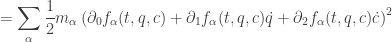
![\displaystyle{ \begin{aligned} &\frac{\partial L}{\partial q_{\alpha i}} \\ &= \frac{\partial}{\partial q_{\alpha i}} \left[ \sum_\alpha \frac{1}{2} m_\alpha \left( \frac{\partial f_\alpha}{\partial t} + \sum_j \frac{\partial f_\alpha}{\partial q_{\alpha j}} \dot q_{\alpha j} + \sum_\beta \frac{\partial f_\alpha}{\partial c_{\alpha \beta}} \dot c_{\alpha \beta} \right)^2 - V(t, f) \right] - 0 \\ &= \sum_\alpha \frac{1}{2} m_\alpha \frac{\partial}{\partial q_{\alpha i}} \left( G \right)^2 - \frac{\partial}{\partial q_{\alpha i}} V(t, f(t;\{q_{\alpha j}\}, \{c_{\alpha \beta}\})) \\ &= \sum_\alpha m_\alpha G \frac{\partial G}{\partial q_{\alpha i}} - \frac{\partial V}{\partial q_{\alpha i}} \\ \end{aligned}}](https://s0.wp.com/latex.php?latex=%5Cdisplaystyle%7B+%5Cbegin%7Baligned%7D+++%26%5Cfrac%7B%5Cpartial+L%7D%7B%5Cpartial+q_%7B%5Calpha+i%7D%7D+%5C%5C++++%26%3D+%5Cfrac%7B%5Cpartial%7D%7B%5Cpartial+q_%7B%5Calpha+i%7D%7D+++++%5Cleft%5B+%5Csum_%5Calpha+%5Cfrac%7B1%7D%7B2%7D+m_%5Calpha+%5Cleft%28+%5Cfrac%7B%5Cpartial+f_%5Calpha%7D%7B%5Cpartial+t%7D+%2B+%5Csum_j+%5Cfrac%7B%5Cpartial+f_%5Calpha%7D%7B%5Cpartial+q_%7B%5Calpha+j%7D%7D+%5Cdot+q_%7B%5Calpha+j%7D+%2B+%5Csum_%5Cbeta+%5Cfrac%7B%5Cpartial+f_%5Calpha%7D%7B%5Cpartial+c_%7B%5Calpha+%5Cbeta%7D%7D+%5Cdot+c_%7B%5Calpha+%5Cbeta%7D+%5Cright%29%5E2+++++-+V%28t%2C+f%29+%5Cright%5D+-+0+%5C%5C++++%26%3D+++++++%5Csum_%5Calpha+%5Cfrac%7B1%7D%7B2%7D+m_%5Calpha+%5Cfrac%7B%5Cpartial%7D%7B%5Cpartial+q_%7B%5Calpha+i%7D%7D+%5Cleft%28+G+%5Cright%29%5E2+++++-+%5Cfrac%7B%5Cpartial%7D%7B%5Cpartial+q_%7B%5Calpha+i%7D%7D+V%28t%2C+f%28t%3B%5C%7Bq_%7B%5Calpha+j%7D%5C%7D%2C+%5C%7Bc_%7B%5Calpha+%5Cbeta%7D%5C%7D%29%29+++%5C%5C++++%26%3D+++%5Csum_%5Calpha+m_%5Calpha+++++G++++%5Cfrac%7B%5Cpartial+G%7D%7B%5Cpartial+q_%7B%5Calpha+i%7D%7D+++++-+%5Cfrac%7B%5Cpartial+V%7D%7B%5Cpartial+q_%7B%5Calpha+i%7D%7D++++%5C%5C++++++%5Cend%7Baligned%7D%7D&bg=ffffff&fg=333333&s=0&c=20201002)


![\displaystyle{ \begin{aligned} mD^2x(t) + \frac{F(t)}{l} \left[x(t) - x_s(t)\right] &= 0 \\ mg + m D^2y(t) + \frac{F(t)}{l} [y(t) - y_s(t)] &= 0 \\ -l^2 + [y(t)-y_s(t)]^2 + [x(t)-x_s(t)]^2 &= 0 \\ \end{aligned}}](https://s0.wp.com/latex.php?latex=%5Cdisplaystyle%7B+%5Cbegin%7Baligned%7D+++mD%5E2x%28t%29+%2B+%5Cfrac%7BF%28t%29%7D%7Bl%7D+%5Cleft%5Bx%28t%29+-+x_s%28t%29%5Cright%5D+%26%3D+0+%5C%5C+++mg+%2B+m+D%5E2y%28t%29+%2B+%5Cfrac%7BF%28t%29%7D%7Bl%7D+%5By%28t%29+-+y_s%28t%29%5D+%26%3D+0+%5C%5C+++-l%5E2+%2B+%5By%28t%29-y_s%28t%29%5D%5E2+%2B+%5Bx%28t%29-x_s%28t%29%5D%5E2+%26%3D+0+%5C%5C++%5Cend%7Baligned%7D%7D&bg=ffffff&fg=333333&s=0&c=20201002)

![\displaystyle{= \sum_\alpha \frac{1}{2} m_\alpha \dot{\mathbf{x}_\alpha}^2 - V(t, x) - \sum_{\{ \alpha, \beta | \alpha < \beta, \alpha \leftrightarrow \beta \}} \frac{F_{\alpha \beta}}{2 l_{\alpha \beta}} \left[ (\mathbf{x}_\beta - \mathbf{x}_\alpha)^2 - l_{\alpha \beta}^2 \right] }](https://s0.wp.com/latex.php?latex=%5Cdisplaystyle%7B%3D+%5Csum_%5Calpha+%5Cfrac%7B1%7D%7B2%7D+m_%5Calpha+%5Cdot%7B%5Cmathbf%7Bx%7D_%5Calpha%7D%5E2++-+V%28t%2C+x%29+-+%5Csum_%7B%5C%7B+%5Calpha%2C+%5Cbeta+%7C+%5Calpha+%3C+%5Cbeta%2C+%5Calpha+%5Cleftrightarrow+%5Cbeta+%5C%7D%7D+%5Cfrac%7BF_%7B%5Calpha+%5Cbeta%7D%7D%7B2+l_%7B%5Calpha+%5Cbeta%7D%7D+%5Cleft%5B+%28%5Cmathbf%7Bx%7D_%5Cbeta+-+%5Cmathbf%7Bx%7D_%5Calpha%29%5E2+-+l_%7B%5Calpha+%5Cbeta%7D%5E2+%5Cright%5D+%7D&bg=ffffff&fg=333333&s=0&c=20201002)
![\displaystyle{ L = \frac{1}{2} m \left[(Dx)^2 + (Dy)^2 \right] - mgy - \frac{F}{2l} \left[ (x-x_s)^2 + (y-y_s)^2 - l^2 \right] }](https://s0.wp.com/latex.php?latex=%5Cdisplaystyle%7B+++++L+++++%3D+++++%5Cfrac%7B1%7D%7B2%7D+m+%5Cleft%5B%28Dx%29%5E2+%2B+%28Dy%29%5E2+%5Cright%5D+-+mgy+++++-+%5Cfrac%7BF%7D%7B2l%7D+%5Cleft%5B+%28x-x_s%29%5E2+%2B+%28y-y_s%29%5E2+-+l%5E2+%5Cright%5D+%7D&bg=ffffff&fg=333333&s=0&c=20201002)


 ) for the system described with the irredundant generalized coordinates
  ,
,  ,
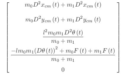
,  and compute the Lagrange equations from this Lagrangian. They should be the same equations as you derived for the same coordinates in part d.

![\displaystyle{ - V(t, f(t,q,c)) - \sum_{\{ \alpha, \beta | \alpha < \beta, \alpha \leftrightarrow \beta \}} \frac{F_{\alpha \beta}}{2 l_{\alpha \beta}} \left[ c_{\alpha \beta}^2 - l_{\alpha \beta}^2 \right] }](https://s0.wp.com/latex.php?latex=%5Cdisplaystyle%7B+++-+V%28t%2C+f%28t%2Cq%2Cc%29%29+-+%5Csum_%7B%5C%7B+%5Calpha%2C+%5Cbeta+%7C+%5Calpha+%3C+%5Cbeta%2C+%5Calpha+%5Cleftrightarrow+%5Cbeta+%5C%7D%7D+++%5Cfrac%7BF_%7B%5Calpha+%5Cbeta%7D%7D%7B2+l_%7B%5Calpha+%5Cbeta%7D%7D+++%5Cleft%5B+++c_%7B%5Calpha+%5Cbeta%7D%5E2+-+l_%7B%5Calpha+%5Cbeta%7D%5E2++%5Cright%5D++%7D&bg=ffffff&fg=333333&s=0&c=20201002)

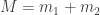
 of, say, three arguments, and let
  be a function of two arguments satisfying
  .
.  .
.  we can set
  and
and  in the Lagrangian, but we cannot do this in deriving the Lagrange equations associated with
  , because we have to take derivatives with respect to those arguments.


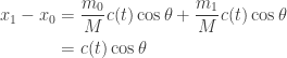
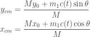
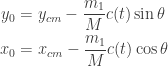
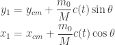
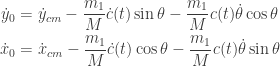
![\displaystyle{ = \frac{1}{2} (m_0 + m_1) (\dot x_{CM}^2 + \dot y_{CM}^2 ) + \frac{1}{2} \left[ m_1 \left( \frac{m_2 l}{m_1 + m_2} \right)^2 + m_2 \left( \frac{m_1 l}{m_1 + m_2} \right)^2 \right] \dot \theta^2 }](https://s0.wp.com/latex.php?latex=%5Cdisplaystyle%7B+%3D+%5Cfrac%7B1%7D%7B2%7D+%28m_0+%2B+m_1%29+%28%5Cdot+x_%7BCM%7D%5E2+%2B+%5Cdot+y_%7BCM%7D%5E2+%29+%2B+%5Cfrac%7B1%7D%7B2%7D+%5Cleft%5B+m_1+%5Cleft%28+%5Cfrac%7Bm_2+l%7D%7Bm_1+%2B+m_2%7D+%5Cright%29%5E2+%2B+m_2+%5Cleft%28+%5Cfrac%7Bm_1+l%7D%7Bm_1+%2B+m_2%7D+%5Cright%29%5E2+%5Cright%5D+%5Cdot+%5Ctheta%5E2+%7D&bg=ffffff&fg=333333&s=0&c=20201002)


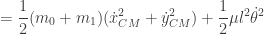

![\displaystyle{ = \frac{1}{2} m_0 \left( \dot x_0^2 + \dot y_0^2 \right) + \frac{1}{2} m_1 \left( \dot x_1^2 + \dot y_1^2 \right) - \frac{F}{2 l} \left[ (y_1 - y_0)^2 + (x_1 - x_0)^2 - l^2 \right] }](https://s0.wp.com/latex.php?latex=%5Cdisplaystyle%7B+%3D+%5Cfrac%7B1%7D%7B2%7D+m_0+%5Cleft%28+%5Cdot+x_0%5E2+%2B+%5Cdot+y_0%5E2+%5Cright%29+%2B+%5Cfrac%7B1%7D%7B2%7D+m_1+%5Cleft%28+%5Cdot+x_1%5E2+%2B+%5Cdot+y_1%5E2+%5Cright%29+-+%5Cfrac%7BF%7D%7B2+l%7D+%5Cleft%5B+%28y_1+-+y_0%29%5E2+%2B+%28x_1+-+x_0%29%5E2+-+l%5E2+%5Cright%5D+%7D&bg=ffffff&fg=333333&s=0&c=20201002)


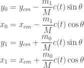


 and
and  ,
,

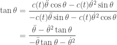


 and since
  ,
,
 and
and  cannot be both zero at the same time,


![\displaystyle{ = \frac{1}{2} m_0 \left( \dot x_0^2 + \dot y_0^2 \right) + \frac{1}{2} m_1 \left( \dot x_1^2 + \dot y_1^2 \right) - \frac{F}{2 l} \left[ (y_1 - y_0)^2 + (x_1 - x_0)^2 - l^2 \right] }](https://s0.wp.com/latex.php?latex=%5Cdisplaystyle%7B++%3D+%5Cfrac%7B1%7D%7B2%7D+m_0+%5Cleft%28+%5Cdot+x_0%5E2+%2B+%5Cdot+y_0%5E2+%5Cright%29++%2B+%5Cfrac%7B1%7D%7B2%7D+m_1+%5Cleft%28+%5Cdot+x_1%5E2+%2B+%5Cdot+y_1%5E2+%5Cright%29++-+%5Cfrac%7BF%7D%7B2+l%7D+%5Cleft%5B+%28y_1+-+y_0%29%5E2+%2B+%28x_1+-+x_0%29%5E2+-+l%5E2+%5Cright%5D++%7D&bg=ffffff&fg=333333&s=0&c=20201002)


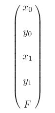


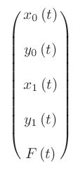
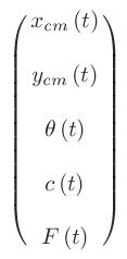
 ,
,  , angle
  , distance between the particles
  , and tension force
  . Write the Lagrangian in these coordinates, and write the Lagrange equations.
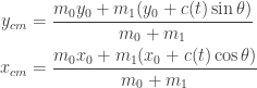
 .
.
![\displaystyle{ \begin{aligned} L &= \frac{1}{2} m_0 (\dot x_0^2 + \dot y_0^2) + \frac{1}{2} m_1 (\dot x_1^2 + \dot y_1^2) + \lambda \left[ (x_1(t) - x_0(t))^2 + (y_1(t) - y_0(t))^2 - l^2 \right] \\ &= \frac{1}{2} m_0 (\dot x_0^2 + \dot y_0^2) + \frac{1}{2} m_1 (\dot x_1^2 + \dot y_1^2) - \frac{F}{2l} \left[ (c(t))^2 - l^2 \right] \\ \end{aligned}}](https://s0.wp.com/latex.php?latex=%5Cdisplaystyle%7B+%5Cbegin%7Baligned%7D+++L+%26%3D+%5Cfrac%7B1%7D%7B2%7D+m_0+%28%5Cdot+x_0%5E2+%2B+%5Cdot+y_0%5E2%29+%2B+%5Cfrac%7B1%7D%7B2%7D+m_1+%28%5Cdot+x_1%5E2+%2B+%5Cdot+y_1%5E2%29+%2B+%5Clambda+%5Cleft%5B+%28x_1%28t%29+-+x_0%28t%29%29%5E2+%2B+%28y_1%28t%29+-+y_0%28t%29%29%5E2+-+l%5E2+%5Cright%5D+%5C%5C+++++%26%3D+%5Cfrac%7B1%7D%7B2%7D+m_0+%28%5Cdot+x_0%5E2+%2B+%5Cdot+y_0%5E2%29+%2B+%5Cfrac%7B1%7D%7B2%7D+m_1+%28%5Cdot+x_1%5E2+%2B+%5Cdot+y_1%5E2%29+++-+%5Cfrac%7BF%7D%7B2l%7D+%5Cleft%5B+%28c%28t%29%29%5E2+-+l%5E2+%5Cright%5D+%5C%5C+++%5Cend%7Baligned%7D%7D&bg=ffffff&fg=333333&s=0&c=20201002)

You must be logged in to post a comment.