SICMUtils

Posted on July 27, 2022 by rpflee

A Clojure(script) implementation of the scmutils system for math and physics investigations in the Clojure and Clojurescript languages.

1. To install Clojure in Ubuntu, just this command is enough:

sudo apt-get install elpa-cider

Although the Clojure version you get is probably not the most updated one, that is not important, because you can specify which version you want in the config file of each project.

2. Then use this command to generate a new project named my-stuff:

lein new app my-stuff

3. Use Emacs to open the file:

~/my-stuff/project.clj

4. Replace the existing :dependencies line with this one

  :dependencies [[org.clojure/clojure "1.11.1"]
                 [sicmutils "0.22.0"]]

And make sure that both clojure and sicmutils have the most updated version numbers.

5. In Emacs, type the command

M-x cider-jack-in

6. In the clojure window (cider-repl), type

(clojure-version)

with enter at the end.

7. Type

(require '[sicmutils.env :as env])

8. Type

(env/bootstrap-repl!)

9. Code

((D cube) 'x)

will result

(+ (* x x) (* x (+ x x)))

10. Type the Emacs command

M-p

to access the last input. Then modify it into

(simplify ((D cube) 'x))

It will result

(* 3 (expt x 2))

11. Code

(->TeX (simplify ((D cube) 'x)))

will give the $LaTeX$ code

3\\,{x}^{2}

12. You can exit by the Emacs command

<C-c C-q>

For the time being, SICMUtils is not suitable for the book SICM (Structure and Interpretation of Classical Mechanics). In other words, SICMUtils cannot replace the scmutils library yet, because:

a. You would have to do the translation manually, from the scmutils code in the book to SICMUtils.

b. Although it can generate $LaTeX$ source code, it does NOT do the $LaTeX$ rendering.

c. It cannot plot graphs.

However, SICMUtils has one advantage over scmutils. It can generate $LaTeX$ source of an expression, but scmutils cannot. So I am planning to use both scmutils and SICMUtils.

Also, I will learn how to use SICMUtils with other Clojure libraries and the Jupyter Notebook. That would get $LaTeX$ rendering and graph plotting running.

— Me@2022-07-26 11:03:51 AM

Common Lisp Reloaded

Posted on July 23, 2022 by rpflee

; sudo apt-get install sbcl

; sudo apt-get install slime

;;;;;;;;;;;;;;;;;;;;;;;;;;;;;;;;;;;;;;;;;;;;;;

(setq inferior-lisp-program "sbcl")

(defun load-slime-with-correct-buffer-position ()

  (save-excursion (slime))
     
 
  (delete-other-windows) 
) 

(defun prelude-start-slime ()
  (unless (slime-connected-p)
    (load-slime-with-correct-buffer-position)))

(add-hook 'slime-mode-hook 'prelude-start-slime)

(set-register ?f '(file . "/path_to/lisp_file.lisp"))

— Me@2022-07-23 05:20:32 PM

Cyclic coordinate

Posted on July 22, 2022 by rpflee

A generalized coordinate component that does not appear explicitly in the Lagrangian is called a cyclic coordinate. The generalized momentum component conjugate to any cyclic coordinate is a constant of the motion.

— 1.8 Conserved Quantities

— Structure and Interpretation of Classical Mechanics

This is a special case of Noether’s theorem. Such coordinates are called “cyclic” or “ignorable”.

— Wikipedia on Lagrangian mechanics

If only the cyclic coordinate $\displaystyle{q(t)}$ varies with time (if it doesn’t, $\displaystyle{q}$ is superfluous), the Lagrangian, or the essential physical situation, doesn’t vary. Hence the initial value of $\displaystyle{q}$ doesn’t determine the path, which is only possible if the path is closed.

— edited Jul 28, 2014 at 15:55

— ACuriousMind

— answered Jul 28, 2014 at 15:50

— Pieter Kockx

— Why are they called “cyclic” coordinates?

— Physics Stack Exchange

2022.07.22 Friday ACHK

Functional programming jargon in plain English

Posted on July 17, 2022 by rpflee

mjburgess 11 days ago | next [–]

These definitions don’t really give you the idea, rather often just code examples..
“The ideas”, in my view:


Monoid	=	units that can be joined together
Functor	=	context for running a single-input function
Applicative	=	context for multi-input functions
Monad	=	context for sequence-dependent operations
Lifting	=	converting from one context to another
Sum type	=	something is either A or B or C…
Product type	=	a record
	=	something is both A and B and C
Partial application	=	defaulting an argument to a function
Currying	=	passing some arguments later
	=	rephrasing a function to return a functions of n-1 arguments when given 1, st. the final function will compute the desired result
EDIT: Context	=	compiler information that changes how the program will be interpreted (, executed, compiled,…)
Eg., context	=	run in the future, run across a list, redirect the i/o, …

— Functional programming jargon in plain English

— Hacker News

Currying and partial function application are often conflated. One of the significant differences between the two is that a call to a partially applied function returns the result right away, not another function down the currying chain; this distinction can be illustrated clearly for functions whose arity is greater than two.

Partial application can be seen as evaluating a curried function at a fixed point, e.g. given $\displaystyle{f\colon (X\times Y\times Z)\to N}$ and $\displaystyle{a\in X}$ then

$\displaystyle{{\text{curry}}({\text{partial}}(f)_{a})(y)(z)={\text{curry}}(f)(a)(y)(z)}$

or simply

$\displaystyle{{\text{partial}}(f)_{a}={\text{curry}}_{1}(f)(a)}$

where $\displaystyle{{\text{curry}}_{1}}$ curries $\displaystyle{f}$ ‘s first parameter.

— Wikipedia on Currying

2022.07.16 Saturday ACHK

Matrix calculus

Posted on July 13, 2022 by rpflee

1.7 Evolution of Dynamical State, 2.3

Structure and Interpretation of Classical Mechanics

$\displaystyle{ \begin{aligned} \partial_1 L \circ \Gamma[q] &= D ( \partial_2 L \circ \Gamma[q]) \\ \\ &= \partial_0 ( \partial_2 L \circ \Gamma[q]) Dt + \partial_1 ( \partial_2 L \circ \Gamma[q]) Dq + \partial_2 ( \partial_2 L \circ \Gamma[q]) Dv \\ \\ &= \partial_0 \partial_2 L \circ \Gamma[q] + ( \partial_1 \partial_2 L \circ \Gamma[q]) Dq + (\partial_2 \partial_2 L \circ \Gamma[q]) D^2 q \\ \\ \end{aligned}}$

$\displaystyle{ \begin{aligned} (\partial_2 \partial_2 L \circ \Gamma[q]) D^2 q &= \partial_1 L \circ \Gamma[q] - \partial_0 \partial_2 L \circ \Gamma[q] - (\partial_1 \partial_2 L \circ \Gamma[q]) Dq \\ \\ D^2 q &= \left[ \partial_2 \partial_2 L \circ \Gamma[q] \right]^{-1} \left\{ \partial_1 L \circ \Gamma[q] - \partial_0 \partial_2 L \circ \Gamma[q] - (\partial_1 \partial_2 L \circ \Gamma[q]) Dq \right\} \\ \\ \end{aligned}}$

where $\displaystyle{\left[ \partial_2 \partial_2 L \circ \Gamma \right]}$ is a structure that can be represented by a symmetric square matrix, so we can compute its inverse.

~~~

[guess]

$\displaystyle{ \begin{aligned} D \left( \frac{\partial}{\partial \dot q_1} L \circ \Gamma[\begin{bmatrix} q_1 \\ q_2 \\ \vdots \end{bmatrix}] \right) - \left(\frac{\partial}{\partial q_1} L \circ \Gamma[\begin{bmatrix} q_1 \\ q_2 \\ \vdots \end{bmatrix}]\right) &= 0 \\ D \left( \frac{\partial}{\partial \dot q_2} L \circ \Gamma[\begin{bmatrix} q_1 \\ q_2 \\ \vdots \end{bmatrix}] \right) - \left(\frac{\partial}{\partial q_2} L \circ \Gamma[\begin{bmatrix} q_1 \\ q_2 \\ \vdots \end{bmatrix}]\right) &= 0 \\ &\vdots \\ \end{aligned}}$

$\displaystyle{ \begin{aligned} D \left( \frac{\partial}{\partial \dot q_1} L \circ \Gamma[\vec q] \right) - \left(\frac{\partial}{\partial q_1} L \circ \Gamma[\vec q]\right) &= 0 \\ D \left( \frac{\partial}{\partial \dot q_2} L \circ \Gamma[\vec q] \right) - \left(\frac{\partial}{\partial q_2} L \circ \Gamma[\vec q]\right) &= 0 \\ &\vdots \\ \end{aligned}}$

$\displaystyle{ \begin{aligned} D \left( \vec \partial_2 L \circ \Gamma[\vec q] \right) - \left(\vec \partial_1 L \circ \Gamma[\vec q]\right) &= 0 \\ \end{aligned}}$

$\displaystyle{ \begin{aligned} \partial_{\vec 1} = \frac{\partial}{\partial \vec q} &= \begin{bmatrix} \frac{\partial}{\partial q_1} & \frac{\partial}{\partial q_2} & ... \end{bmatrix} \\ \\ \partial_{\vec 2} = \frac{\partial}{\partial \vec{\dot q}} &= \begin{bmatrix} \frac{\partial}{\partial \dot q_1} & \frac{\partial}{\partial \dot q_2} & ... \end{bmatrix} \\ \end{aligned}}$

$\displaystyle{ \begin{aligned} \vec \partial_{1} = \left( \frac{\partial}{\partial \vec q} \right)^T &= \begin{bmatrix} \frac{\partial}{\partial q_1} \\ \frac{\partial}{\partial q_2} \\ \vdots \end{bmatrix} \\ \\ \vec \partial_{2} = \left( \frac{\partial}{\partial \vec{\dot q}} \right)^T &= \begin{bmatrix} \frac{\partial}{\partial \dot q_1} \\ \frac{\partial}{\partial \dot q_2} \\ \vdots \end{bmatrix} \\ \end{aligned}}$

$\displaystyle{ \begin{aligned} \vec \partial_1 L \circ \Gamma[\vec q] &= D \left( \vec \partial_2 L \circ \Gamma[\vec q] \right) \\ \\ &= \partial_0 \left( \vec \partial_2 L \circ \Gamma[\vec q] \right) Dt \\ &+ \partial_{q_1} \left( \vec \partial_2 L \circ \Gamma[\vec q] \right) Dq_1 + \partial_{\dot q_1} \left( \vec \partial_2 L \circ \Gamma[\vec q] \right) D \dot q_1 \\ &+ \partial_{q_2} \left( \vec \partial_2 L \circ \Gamma[\vec q] \right) Dq_2 + \partial_{\dot q_2} \left( \vec \partial_2 L \circ \Gamma[\vec q] \right) D \dot q_2 \\ &+ ... \\ \\ &= \partial_0 \left( \vec \partial_2 L \circ \Gamma[\vec q] \right) \\ &+ \begin{bmatrix} \partial_{q_1} & \partial_{q_2} & ... \end{bmatrix} \left( \vec \partial_2 L \circ \Gamma[\vec q] \right) D \begin{bmatrix} q_1 \\ q_2 \\ \vdots \end{bmatrix} \\ &+ \begin{bmatrix} \partial_{\dot q_1} & \partial_{\dot q_2} & ... \end{bmatrix} \left( \vec \partial_2 L \circ \Gamma[\vec q] \right) D^2 \begin{bmatrix} q_1 \\ q_2 \\ \vdots \end{bmatrix} \\ \end{aligned}}$

$\displaystyle{\begin{aligned} \vec \partial_1 L \circ \Gamma[\vec q] &= \partial_0 \left( \vec \partial_2 L \circ \Gamma[\vec q] \right) Dt + \frac{\partial}{\partial \vec q} \left( \vec \partial_2 L \circ \Gamma[\vec q] \right) D \vec q + \frac{\partial}{\partial \vec {\dot q}} \left( \vec \partial_2 L \circ \Gamma[\vec q] \right) D^2 \vec q \\ \end{aligned}}$

[guess]

— Me@2022-07-09 09:09:28 PM

Common Lisp vs Racket

Posted on July 13, 2022 by rpflee

flavio81 11 months ago [-]

The author, a famous and well-liked lisper, is not considering portability features. CL is an ANSI standard and code often runs with no changes in many distinct CL implementations/compilers/interpreters.

Also, related to that point: There are many different CL implementations out there that satisfy different use cases, like for example JVM deployment (ABCL), embedded systems (ECL), speed(SBCL), fast compile times (Clozure), pro-level support (LispWorks, ACL), etc. So the same code has a huge amount of options for deployment. It really makes Common Lisp be “write once, run anywhere”.

Then speed is also never mentioned. Lisp can be seriously fast; under SBCL it is generally 0.3x to 1x C speed; LispWorks might be faster, and there’s a PDF out there called “How to make Lisp go faster than C”, so that should give an idea of Lisp speed potential.

CL wasn’t created by philosophing about what a programming language should be for many years; CL was basically created by merging Lisps that were already proven in the industry (Maclisp, Zetalisp, etc), already proven to be good for AI, heavy computation, symbolic computation, launching rockets, writing full operating systems, etc.

CL is a “you want it, you got it” programming language. You want to circumvent the garbage collector? Need to use GOTOs for a particular function? Want to produce better assembly out? Need side effects? Multiple inheritance? Want to write an OS? CL will deliver the goods.

In short, I would guess that from a computer scientist or reseacher point of view, Racket is certainly more attactive, but for the engineer or start-up owner that wants to have killer production systems done in short time, or to create really complex, innovative systems that can be deployed to the real world, Common Lisp ought to be the weapon of choice!

— Why I haven’t jumped ship from Common Lisp to Racket just yet

— Hacker News

2022.07.13 Wednesday ACHK

1.7 Evolution of Dynamical State, 2.2

Posted on July 9, 2022 by rpflee

Structure and Interpretation of Classical Mechanics

where $\displaystyle{\left[ \partial_2 \partial_2 L \circ \Gamma \right]}$ is a structure that can be represented by a symmetric square matrix, so we can compute its inverse.

~~~

[guess]

The Lagrange equation:

$\displaystyle{ \begin{aligned} D \left( \frac{\partial}{\partial \dot q_1} L \circ \Gamma[\begin{bmatrix} q_1 \\ q_2 \end{bmatrix}] \right) - \left(\frac{\partial}{\partial q_1} L \circ \Gamma[\begin{bmatrix} q_1 \\ q_2 \end{bmatrix}]]\right) &= 0 \\ \end{aligned}}$

$\displaystyle{ \begin{aligned} D \left( \frac{\partial}{\partial \dot q_2} L \circ \Gamma[\begin{bmatrix} q_1 \\ q_2 \end{bmatrix}]] \right) - \left(\frac{\partial}{\partial q_2} L \circ \Gamma[\begin{bmatrix} q_1 \\ q_2 \end{bmatrix}]]\right) &= 0 \\ \end{aligned}}$

$\displaystyle{ \begin{aligned} \frac{d}{dt} \left( \frac{\partial}{\partial \dot q_1} L (t, q_1(t), \dot q_1(t), q_2(t), \dot q_2(t)) \right) - \frac{\partial}{\partial q_1} L (t, q_1(t), \dot q_1(t), q_2(t), \dot q_2(t)) &= 0 \end{aligned}}$

$\displaystyle{ \begin{aligned} \frac{d}{dt} \left( \frac{\partial}{\partial \dot q_2} L (t, q_1(t), \dot q_1(t), q_2(t), \dot q_2(t)) \right) - \frac{\partial}{\partial q_2} L (t, q_1(t), \dot q_1(t), q_2(t), \dot q_2(t)) &= 0 \end{aligned}}$

$\displaystyle{ \begin{aligned} D \left( \begin{bmatrix} \frac{\partial}{\partial \dot q_1} \\ \frac{\partial}{\partial \dot q_2} \end{bmatrix} L \circ \Gamma[q_1, q_2] \right) - \left( \begin{bmatrix} \frac{\partial}{\partial q_1} \\ \frac{\partial}{\partial q_2} \end{bmatrix} L \circ \Gamma[q_1, q_2]\right) &= 0 \\ D \left( \vec \partial_2 L \circ \Gamma[q_1, q_2] \right) - \left( \vec \partial_1 L \circ \Gamma[q_1, q_2]\right) &= 0 \\ \end{aligned}}$

$\displaystyle{ \begin{aligned} \vec \partial_1 L \circ \Gamma[q] &= D ( \vec \partial_2 L \circ \Gamma[q]) \\ \\ \begin{bmatrix} \frac{\partial}{\partial q_1} \\ \frac{\partial}{\partial q_2} \end{bmatrix} L \circ \Gamma[q_1, q_2] &= D \left( \begin{bmatrix} \frac{\partial}{\partial \dot q_1} \\ \frac{\partial}{\partial \dot q_2} \end{bmatrix} L \circ \Gamma[q_1, q_2] \right) \\ \\ \frac{\partial}{\partial q_1} L \circ \Gamma[q_1, q_2] &= \partial_0 \left(\frac{\partial}{\partial \dot q_1} L \circ \Gamma[q_1, q_2] \right) Dt \\ &+ \partial_{q_1} \left(\frac{\partial}{\partial \dot q_1} L \circ \Gamma[q_1, q_2] \right) D q_1 + \partial_{v_1} \left(\frac{\partial}{\partial \dot q_1} L \circ \Gamma[q_1, q_2] \right) D v_1 \\ &+ \partial_{q_2} \left(\frac{\partial}{\partial \dot q_1} L \circ \Gamma[q_1, q_2] \right) D q_2 + \partial_{v_2} \left(\frac{\partial}{\partial \dot q_1} L \circ \Gamma[q_1, q_2] \right) D v_2 \\ \frac{\partial}{\partial q_2} L \circ \Gamma[q_1, q_2] &= ... \\ \end{aligned}}$

$\displaystyle{ \begin{aligned} \frac{\partial}{\partial q_1} L \circ \Gamma[q_1, q_2] &= \partial_0 \left(\frac{\partial}{\partial \dot q_1} L \circ \Gamma[q_1, q_2] \right) Dt \\ &+ \frac{\partial}{\partial q_1} \left(\frac{\partial}{\partial \dot q_1} L \circ \Gamma[q_1, q_2] \right) D q_1 + \frac{\partial}{\partial q_2} \left(\frac{\partial}{\partial \dot q_1} L \circ \Gamma[q_1, q_2] \right) D q_2 \\ &+ \frac{\partial}{\partial \dot q_1} \left(\frac{\partial}{\partial \dot q_1} L \circ \Gamma[q_1, q_2] \right) D^2 q_1 + \frac{\partial}{\partial \dot q_2} \left(\frac{\partial}{\partial \dot q_1} L \circ \Gamma[q_1, q_2] \right) D^2 q_2 \\ \frac{\partial}{\partial q_2} L \circ \Gamma[q_1, q_2] &= \partial_0 \left(\frac{\partial}{\partial \dot q_2} L \circ \Gamma[q_1, q_2] \right) Dt \\ &+ \frac{\partial}{\partial q_1} \left(\frac{\partial}{\partial \dot q_2} L \circ \Gamma[q_1, q_2] \right) D q_1 + \frac{\partial}{\partial q_2} \left(\frac{\partial}{\partial \dot q_2} L \circ \Gamma[q_1, q_2] \right) D q_2 \\ &+ \frac{\partial}{\partial \dot q_1} \left(\frac{\partial}{\partial \dot q_2} L \circ \Gamma[q_1, q_2] \right) D^2 q_1 + \frac{\partial}{\partial \dot q_2} \left(\frac{\partial}{\partial \dot q_2} L \circ \Gamma[q_1, q_2] \right) D^2 q_2 \\ \end{aligned}}$

$\displaystyle{\begin{aligned} \vec \partial_1 L \circ \Gamma[q_1, q_2] &= \partial_0 \left(\vec \partial_2 L \circ \Gamma[q_1, q_2] \right) Dt \\ &+ \frac{\partial}{\partial q_1} \left( \vec \partial_2 L \circ \Gamma[q_1, q_2] \right) D q_1 + \frac{\partial}{\partial q_2} \left( \vec \partial_2 L \circ \Gamma[q_1, q_2] \right) D q_2 \\ &+ \frac{\partial}{\partial \dot q_1} \left( \vec \partial_2 L \circ \Gamma[q_1, q_2] \right) D^2 q_1 + \frac{\partial}{\partial \dot q_2} \left( \vec \partial_2 L \circ \Gamma[q_1, q_2] \right) D^2 q_2 \\ \\ \end{aligned}}$

$\displaystyle{\begin{aligned} \begin{bmatrix} \frac{\partial}{\partial q_1} \\ \frac{\partial}{\partial q_2} \end{bmatrix} L \circ \Gamma[q_1, q_2] &= \partial_0 \left( \begin{bmatrix} \frac{\partial}{\partial \dot q_1} \\ \frac{\partial}{\partial \dot q_2} \end{bmatrix} L \circ \Gamma[q_1, q_2] \right) Dt \\ &+ \frac{\partial}{\partial q_1} \left( \begin{bmatrix} \frac{\partial}{\partial \dot q_1} \\ \frac{\partial}{\partial \dot q_2} \end{bmatrix} L \circ \Gamma[q_1, q_2] \right) D q_1 + \frac{\partial}{\partial q_2} \left( \begin{bmatrix} \frac{\partial}{\partial \dot q_1} \\ \frac{\partial}{\partial \dot q_2} \end{bmatrix} L \circ \Gamma[q_1, q_2] \right) D q_2 \\ &+ \frac{\partial}{\partial \dot q_1} \left( \begin{bmatrix} \frac{\partial}{\partial \dot q_1} \\ \frac{\partial}{\partial \dot q_2} \end{bmatrix} L \circ \Gamma[q_1, q_2] \right) D^2 q_1 + \frac{\partial}{\partial \dot q_2} \left( \begin{bmatrix} \frac{\partial}{\partial \dot q_1} \\ \frac{\partial}{\partial \dot q_2} \end{bmatrix} L \circ \Gamma[q_1, q_2] \right) D^2 q_2 \\ \\ \end{aligned}}$

$\displaystyle{ \begin{aligned} \frac{\partial}{\partial \dot q_1} \left(\frac{\partial}{\partial \dot q_1} L \circ \Gamma[\vec q] \right) D^2 q_1 + \frac{\partial}{\partial \dot q_2} \left(\frac{\partial}{\partial \dot q_1} L \circ \Gamma[\vec q] \right) D^2 q_2 &= \frac{\partial}{\partial q_1} L \circ \Gamma[\vec q] - \partial_0 \left(\frac{\partial}{\partial \dot q_1} L \circ \Gamma[\vec q] \right) Dt \\ &- \frac{\partial}{\partial q_1} \left(\frac{\partial}{\partial \dot q_1} L \circ \Gamma[\vec q] \right) D q_1 - \frac{\partial}{\partial q_2} \left(\frac{\partial}{\partial \dot q_1} L \circ \Gamma[\vec q] \right) D q_2 \\ \\ \frac{\partial}{\partial \dot q_1} \left(\frac{\partial}{\partial \dot q_2} L \circ \Gamma[\vec q] \right) D^2 q_1 + \frac{\partial}{\partial \dot q_2} \left(\frac{\partial}{\partial \dot q_2} L \circ \Gamma[\vec q] \right) D^2 q_2 &= \frac{\partial}{\partial q_2} L \circ \Gamma[\vec q] - \partial_0 \left(\frac{\partial}{\partial \dot q_2} L \circ \Gamma[\vec q] \right) Dt \\ &- \frac{\partial}{\partial q_1} \left(\frac{\partial}{\partial \dot q_2} L \circ \Gamma[\vec q] \right) D q_1 - \frac{\partial}{\partial q_2} \left(\frac{\partial}{\partial \dot q_2} L \circ \Gamma[\vec q] \right) D q_2 \\ \end{aligned}}$

$\displaystyle{ \begin{aligned} &\begin{bmatrix} \frac{\partial}{\partial \dot q_1} \left(\frac{\partial}{\partial \dot q_1} L \circ \Gamma[\vec q] \right) & \frac{\partial}{\partial \dot q_2} \left(\frac{\partial}{\partial \dot q_1} L \circ \Gamma[\vec q] \right) \\ \frac{\partial}{\partial \dot q_1} \left(\frac{\partial}{\partial \dot q_2} L \circ \Gamma[\vec q] \right) & \frac{\partial}{\partial \dot q_2} \left(\frac{\partial}{\partial \dot q_2} L \circ \Gamma[\vec q] \right) \end{bmatrix} \begin{bmatrix} D^2 q_1 \\ D^2 q_2 \end{bmatrix} \\ &= \begin{bmatrix} \frac{\partial}{\partial q_1} L \circ \Gamma[\vec q] - \partial_0 \left(\frac{\partial}{\partial \dot q_1} L \circ \Gamma[\vec q] \right) Dt - \frac{\partial}{\partial q_1} \left(\frac{\partial}{\partial \dot q_1} L \circ \Gamma[\vec q] \right) D q_1 - \frac{\partial}{\partial q_2} \left(\frac{\partial}{\partial \dot q_1} L \circ \Gamma[\vec q] \right) D q_2 \\ \\ \frac{\partial}{\partial q_2} L \circ \Gamma[\vec q] - \partial_0 \left(\frac{\partial}{\partial \dot q_2} L \circ \Gamma[\vec q] \right) Dt - \frac{\partial}{\partial q_1} \left(\frac{\partial}{\partial \dot q_2} L \circ \Gamma[\vec q] \right) D q_1 - \frac{\partial}{\partial q_2} \left(\frac{\partial}{\partial \dot q_2} L \circ \Gamma[\vec q] \right) D q_2 \\ \end{bmatrix} \end{aligned}}$

$\displaystyle{ \begin{aligned} &\left(\begin{bmatrix} \frac{\partial}{\partial \dot q_1} \left(\frac{\partial}{\partial \dot q_1} \right) & \frac{\partial}{\partial \dot q_2} \left(\frac{\partial}{\partial \dot q_1} \right) \\ \frac{\partial}{\partial \dot q_1} \left(\frac{\partial}{\partial \dot q_2} \right) & \frac{\partial}{\partial \dot q_2} \left(\frac{\partial}{\partial \dot q_2} \right) \end{bmatrix} L \circ \Gamma[\vec q] \right)\begin{bmatrix} D^2 q_1 \\ D^2 q_2 \end{bmatrix} \\ &= \begin{bmatrix} \frac{\partial}{\partial q_1} \\ \frac{\partial}{\partial q_2} \end{bmatrix} L \circ \Gamma[\vec q] - \left( \partial_0 \begin{bmatrix} \frac{\partial}{\partial \dot q_1} \\ \frac{\partial}{\partial \dot q_2} \end{bmatrix} L \circ \Gamma[\vec q] \right) Dt - \left( \begin{bmatrix} \frac{\partial}{\partial q_1} \left(\frac{\partial}{\partial \dot q_1} \right) & \frac{\partial}{\partial q_2} \left(\frac{\partial}{\partial \dot q_1} \right) \\ \\ \frac{\partial}{\partial q_1} \left(\frac{\partial}{\partial \dot q_2} \right) & \frac{\partial}{\partial q_2} \left(\frac{\partial}{\partial \dot q_2} \right) \\ \end{bmatrix} L \circ \Gamma[\vec q] \right) \begin{bmatrix} D q_1 \\ D q_2 \end{bmatrix} \\ \end{aligned}}$

$\displaystyle{ \begin{aligned} &\left( \begin{bmatrix} \frac{\partial}{\partial \dot q_1} \\ \frac{\partial}{\partial \dot q_2} \\ \end{bmatrix} \begin{bmatrix} \frac{\partial}{\partial \dot q_1} & \frac{\partial}{\partial \dot q_2} \\ \end{bmatrix} L \circ \Gamma[\vec q] \right)\begin{bmatrix} D^2 q_1 \\ D^2 q_2 \end{bmatrix} \\ &= \begin{bmatrix} \frac{\partial}{\partial q_1} \\ \frac{\partial}{\partial q_2} \end{bmatrix} L \circ \Gamma[\vec q] - \left( \partial_0 \begin{bmatrix} \frac{\partial}{\partial \dot q_1} \\ \frac{\partial}{\partial \dot q_2} \end{bmatrix} L \circ \Gamma[\vec q] \right) Dt - \left( \begin{bmatrix} \frac{\partial}{\partial \dot q_1} \\ \frac{\partial}{\partial \dot q_2} \end{bmatrix} \begin{bmatrix} \frac{\partial}{\partial q_1} & \frac{\partial}{\partial q_2} \end{bmatrix} L \circ \Gamma[\vec q] \right) \begin{bmatrix} D q_1 \\ D q_2 \end{bmatrix} \\ \end{aligned}}$

$\displaystyle{ \begin{aligned} &\left( \vec \partial_2 \vec \partial_2^T L \circ \Gamma[\vec q] \right) D^2 \vec q \\ &= \vec \partial_1 L \circ \Gamma[\vec q] - \left( \partial_0 \vec \partial_2 L \circ \Gamma[\vec q] \right) - \left( \vec \partial_2 \vec \partial_1^T L \circ \Gamma[\vec q] \right) D \vec q \\ \end{aligned}}$

[guess]

— Me@2022-07-07 05:20:38 PM

1.7 Evolution of Dynamical State, 2.1

Posted on July 9, 2022 by rpflee

Structure and Interpretation of Classical Mechanics

where $\displaystyle{\left[ \partial_2 \partial_2 L \circ \Gamma \right]}$ is a structure that can be represented by a symmetric square matrix, so we can compute its inverse.

~~~

[guess]

Eq. (1.110):

$\displaystyle{ \left(D \Gamma[q] \right)(t) = \left( 1, Dq(t), D^2 q(t), ... \right) = \begin{bmatrix} 1 \\ Dq(t) \\ D^2 q(t) \\ ... \\ \end{bmatrix} \\ }$

$\displaystyle{ \Gamma[q](t) = \left( t, q(t), D q(t), D^2 q(t), ... \right) = \begin{bmatrix} t \\ q(t) \\ D q(t) \\ D^2 q(t) \\ ... \\ \end{bmatrix} \\ }$

$\displaystyle{ \Gamma[q] = \begin{bmatrix} I \\ q \\ D q \\ D^2 q \\ ... \\ \end{bmatrix} \\ }$ ,

where $I(t) = t$ .

$\displaystyle{ \Gamma[q_1, q_2](t) = \left( t, \begin{bmatrix} q_1(t) \\ q_2(t) \end{bmatrix}, D \begin{bmatrix} q_1(t) \\ q_2(t) \end{bmatrix}, D^2 \begin{bmatrix} q_1(t) \\ q_2(t) \end{bmatrix}, ... \right) = \begin{bmatrix} t \\ \begin{bmatrix} q_1(t) \\ q_2(t) \end{bmatrix} \\ D \begin{bmatrix} q_1(t) \\ q_2(t) \end{bmatrix} \\ D^2 \begin{bmatrix} q_1(t) \\ q_2(t) \end{bmatrix} \\ ... \\ \end{bmatrix} \\ }$

The Lagrange equation:

$\displaystyle{ \begin{aligned} D ( \partial_2 L \circ \Gamma[q]) - (\partial_1 L \circ \Gamma[q]) &= 0 \\ \end{aligned}}$

$\displaystyle{ \begin{aligned} \frac{d}{dt} \left( \frac{\partial}{\partial \dot q} L (t, q(t), \dot q(t)) \right) - \frac{\partial}{\partial q} L (t, q(t), \dot q(t)) &= 0 \end{aligned}}$

$\displaystyle{ \begin{aligned} D \left( \frac{\partial}{\partial \dot q_1} L \circ \Gamma[q_1, q_2] \right) - \left(\frac{\partial}{\partial q_1} L \circ \Gamma[q_1, q_2]\right) &= 0 \\ \end{aligned}}$

$\displaystyle{ \begin{aligned} D \left( \frac{\partial}{\partial \dot q_2} L \circ \Gamma[q_1, q_2] \right) - \left(\frac{\partial}{\partial q_2} L \circ \Gamma[q_1, q_2]\right) &= 0 \\ \end{aligned}}$

$\displaystyle{ \begin{aligned} \vec \partial_1 L \circ \Gamma[q] &= D ( \vec \partial_2 L \circ \Gamma[q]) \\ \\ \begin{bmatrix} \frac{\partial}{\partial q_1} \\ \frac{\partial}{\partial q_2} \end{bmatrix} L \circ \Gamma[q_1, q_2] &= D \left( \begin{bmatrix} \frac{\partial}{\partial \dot q_1} \\ \frac{\partial}{\partial \dot q_2} \end{bmatrix} L \circ \Gamma[q_1, q_2] \right) \\ \\ \frac{\partial}{\partial q_1} L \circ \Gamma[q_1, q_2] &= D \left(\frac{\partial}{\partial \dot q_1} L \circ \Gamma[q_1, q_2] \right) \\ \frac{\partial}{\partial q_2} L \circ \Gamma[q_1, q_2] &= D \left( \frac{\partial}{\partial \dot q_2} L \circ \Gamma[q_1, q_2] \right) \\ \\ \frac{\partial}{\partial q_1} L \circ \Gamma[q_1, q_2] &= \partial_0 \left(\frac{\partial}{\partial \dot q_1} L \circ \Gamma[q_1, q_2] \right) Dt \\ &+ \partial_{q_1} \left(\frac{\partial}{\partial \dot q_1} L \circ \Gamma[q_1, q_2] \right) D q_1 + \partial_{v_1} \left(\frac{\partial}{\partial \dot q_1} L \circ \Gamma[q_1, q_2] \right) D v_1 \\ &+ \partial_{q_2} \left(\frac{\partial}{\partial \dot q_1} L \circ \Gamma[q_1, q_2] \right) D q_2 + \partial_{v_2} \left(\frac{\partial}{\partial \dot q_1} L \circ \Gamma[q_1, q_2] \right) D v_2 \\ \frac{\partial}{\partial q_2} L \circ \Gamma[q_1, q_2] &= ... \\ \end{aligned}}$

This part is wrong.

$\displaystyle{\begin{aligned} \vec \partial_1 L \circ \Gamma[q_1, q_2] &= \partial_0 \left(\vec \partial_2 L \circ \Gamma[q_1, q_2] \right) Dt \\ &+ \frac{\partial}{\partial q_1} \left( \vec \partial_2 L \circ \Gamma[q_1, q_2] \right) D q_1 + \frac{\partial}{\partial q_2} \left( \vec \partial_2 L \circ \Gamma[q_1, q_2] \right) D q_2 \\ &+ \frac{\partial}{\partial \dot q_1} \left( \vec \partial_2 L \circ \Gamma[q_1, q_2] \right) D^2 q_1 + \frac{\partial}{\partial \dot q_2} \left( \vec \partial_2 L \circ \Gamma[q_1, q_2] \right) D^2 q_2 \\ \\ &= \partial_0 \left(\vec \partial_2 L \circ \Gamma[q_1, q_2] \right) Dt \\ &+ \begin{bmatrix} \frac{\partial}{\partial q_1} & \frac{\partial}{\partial q_2} \\ \end{bmatrix} \begin{bmatrix} \left( \vec \partial_2 L \circ \Gamma[q_1, q_2] \right) D q_1 \\ \left( \vec \partial_2 L \circ \Gamma[q_1, q_2] \right) D q_2 \\ \end{bmatrix} + \begin{bmatrix} \frac{\partial}{\partial \dot q_1} & \frac{\partial}{\partial \dot q_2} \\ \end{bmatrix} \begin{bmatrix} \left( \vec \partial_2 L \circ \Gamma[q_1, q_2] \right) D^2 q_1 \\ \left( \vec \partial_2 L \circ \Gamma[q_1, q_2] \right) D^2 q_2 \\ \end{bmatrix} \\ \\ \end{aligned}}$

$\displaystyle{\begin{aligned} &= \partial_0 \left(\vec \partial_2 L \circ \Gamma[q_1, q_2] \right) Dt \\ &+ \begin{bmatrix} \frac{\partial}{\partial q_1} & \frac{\partial}{\partial q_2} \\ \end{bmatrix} \left( \vec \partial_2 L \circ \Gamma[q_1, q_2] \right) D \begin{bmatrix} q_1 \\ q_2 \\ \end{bmatrix} + \begin{bmatrix} \frac{\partial}{\partial \dot q_1} & \frac{\partial}{\partial \dot q_2} \\ \end{bmatrix} \left( \vec \partial_2 L \circ \Gamma[q_1, q_2] \right) D^2 \begin{bmatrix} q_1 \\ q_2 \\ \end{bmatrix} \\ \\ \vec \partial_1 L \circ \Gamma[\vec q] &= \partial_0 \left(\vec \partial_2 L \circ \Gamma[q_1, q_2] \right) + \vec \partial_1^T \left( \vec \partial_2 L \circ \Gamma[\vec q] \right) D \vec q + \vec \partial_2^T \left( \vec \partial_2 L \circ \Gamma[\vec q] \right) D^2 \vec q \\ \end{aligned}}$

This can be proven wrong by just checking the dimensions of the matrix products.

The source of the errors is the second step. It puts the column matrix $\displaystyle{\vec \partial_2 = \begin{bmatrix} \frac{\partial}{\partial \dot q_1} & \frac{\partial}{\partial \dot q_2} \end{bmatrix}^T}$ into each equation. Instead, each row of $\displaystyle{\vec \partial_2}$ should match only one of the two equations.

[guess]

— Me@2022-07-07 05:20:38 PM

1.7 Evolution of Dynamical State

Posted on June 30, 2022 by rpflee

Lagrange’s equations are ordinary differential equations that the path must
satisfy. They can be used to test if a proposed path is a realizable path of the
system. However, we can also use them to develop a path, starting with initial
conditions.

Assume that the state of a system is given by the tuple $\displaystyle{(t, q, v)}$ . If we are
given a prescription for computing the acceleration $\displaystyle{a = A(t, q, v)}$ , then

$\displaystyle{D^2 q = A \circ \Gamma[q]}$

and we have as a consequence

$\displaystyle{D^3 q = D( A \circ \Gamma[q]) = D_t A \circ \Gamma[q]}$

and so on.

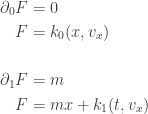
So the higher-derivative components of the local tuple are given by functions $\displaystyle{D_t A, D_t^2 A, \dots}$ . Each of these functions depends on lower-derivative components of the local tuple. All we need to deduce the path from the state is a function that gives the next-higher derivative component of the local description from the state. We use the Lagrange equations to find this function.

— Structure and Interpretation of Classical Mechanics

Eq. (1.113):

$\displaystyle{ D_t F \circ \Gamma[q] = D(F \circ \Gamma[q]) }$

Eq. (1.114):

$\displaystyle{ \begin{aligned} D_t F (t, q, v, a, ...) &= \partial_0 F(t, q, v, a, ...) + \partial_1 F(t, q, v, a, ...) v + \partial_2 F(t, q, v, a, ...) a + ... \\ \end{aligned} }$

$\displaystyle{ \begin{aligned} D_t F \circ \Gamma[q] (t) &= \partial_0 F(t, q, v, a, ...) + \partial_1 F(t, q, v, a, ...) v(t) + \partial_2 F(t, q, v, a, ...) a(t) + ... \\ \end{aligned} }$

The Lagrange equation:

$\displaystyle{ \begin{aligned} \frac{d}{dt} \left( \frac{\partial}{\partial \dot q} L (t, q(t), \dot q(t)) \right) - \frac{\partial}{\partial q} L (t, q(t), \dot q(t)) &= 0 \end{aligned}}$

$\displaystyle{ \begin{aligned} D ( \partial_2 L \circ \Gamma[q]) - (\partial_1 L \circ \Gamma[q]) &= 0 \\ \end{aligned}}$

where $\displaystyle{\left[ \partial_2 \partial_2 L \circ \Gamma \right]}$ is a structure that can be represented by a symmetric square matrix, so we can compute its inverse.

— Me@2022-06-30 11:33:27 AM

C-h ?

Posted on June 19, 2022 by rpflee

C-h w command-name


C-h k key-sequence

C-h f function-name

— Me@2022-06-18 12:52:10 PM

Ex 1.27 Identifying total time derivatives

Posted on June 17, 2022 by rpflee

Structure and Interpretation of Classical Mechanics

From equation (1.112), we see that $\displaystyle{G}$ must be linear in the generalized velocities

$\displaystyle{ G(t, q, v) = G_0(t, q, v) + G_1(t, q, v) v }$

where neither $\displaystyle{G_1}$ nor $\displaystyle{G_0}$ depend on the generalized velocities: $\displaystyle{\partial_2 G_1 = \partial_2 G_0 = 0}$ .

.

So if $\displaystyle{G}$ is the total time derivative of $\displaystyle{F}$ then

$\displaystyle{ \partial_0 G_1 = \partial_1 G_0 }$

…

For each of the following functions, either show that it is not a total time derivative or produce a function from which it can be derived.

~~~

[guess]

a. $\displaystyle{G(t, x, v_x) = m v_x}$

$\displaystyle{ \begin{aligned} G_0 &= 0 \\ G_1 &= m \\ \\ \partial_0 G_1 &= 0 \\ \partial_1 G_0 &= 0 \\ \\ \end{aligned} }$

$\displaystyle{ \begin{aligned} \partial_0 F &= 0 \\ F &= k_0(x, v_x) \\ \\ \partial_1 F &= m \\ F &= m x + k_1(t, v_x) \\ \end{aligned} }$

Let

$\displaystyle{ \begin{aligned} k_0(x, v_x) &= mx \\ k_1(t, v_x) &= 0 \\ \end{aligned} }$

Then

$\displaystyle{ \begin{aligned} F &= mx \\ \end{aligned} }$

[guess]

— Me@2022-06-17 05:10:38 PM

3Blue1Brown

Posted on June 5, 2022 by rpflee

(defun 3b1b ()

    (interactive)

    (setq is-python-mode (string= major-mode "python-mode"))

    (if (not is-python-mode)
        (print "This is not a python file.")


        (print buffer-file-name)

        (setq the-command (format "%s %s %s" 
                                "manim -p"
                                buffer-file-name  
                                "JustAShape")) 

        (print the-command)                        

        (shell-command the-command) 
    )  
)

(global-set-key (kbd "C-p") '3b1b)

(global-set-key (kbd "C-/") 'comment-region)

(global-set-key (kbd "C-.") 'uncomment-region)

— Me@2022-06-05 04:00:37 PM

Ex 1.26 Lagrange equations for total time derivatives

Posted on June 5, 2022 by rpflee

Structure and Interpretation of Classical Mechanics

Let $\displaystyle{F(t, q)}$ be a function of $\displaystyle{t}$ and $\displaystyle{q}$ only, with total time derivative

$\displaystyle{D_t F = \partial_0 F + \partial_1 F \dot Q}$

Show explicitly that the Lagrange equations for $\displaystyle{D_t F}$ are identically zero, …

~~~

[guess]

The Lagrange equation:

$\displaystyle{ \begin{aligned} D ( \partial_2 L \circ \Gamma[q]) - (\partial_1 L \circ \Gamma[q]) &= 0 \\ \end{aligned}}$

$\displaystyle{ \begin{aligned} \frac{d}{dt} \left( \frac{\partial}{\partial \dot q} L (t, q(t), \dot q(t)) \right) - \frac{\partial}{\partial q} L (t, q(t), \dot q(t)) &= 0 \end{aligned}}$

Eq. (1.114):

$\displaystyle{ \begin{aligned} D_t F (t, q, v, a, ...) &= \partial_0 F(t, q, v, a, ...) + \partial_1 F(t, q, v, a, ...) v + \partial_2 F(t, q, v, a, ...) a + ... \\ \end{aligned} }$

$\displaystyle{ \begin{aligned} D_t F \circ \Gamma[q] (t) &= \partial_0 F(t, q, v, a, ...) + \partial_1 F(t, q, v, a, ...) v(t) + \partial_2 F(t, q, v, a, ...) a(t) + ... \\ \end{aligned} }$

Put $\displaystyle{ D_t F (t, q, Dq, ...) }$ into the Lagrange equation:

$\displaystyle{ \begin{aligned} &\frac{d}{dt} \left( \frac{\partial}{\partial \dot q} D_t F (t, q, Dq, ...) \right) - \frac{\partial}{\partial q} D_t F (t, q, Dq, ...) \\ \\ &= \frac{d}{dt} \left[ \frac{\partial}{\partial \dot q} \left( \partial_0 F(t, q, v, a, ...) + \partial_1 F(t, q, v, a, ...) v + \partial_2 F(t, q, v, a, ...) a + ... \right) \right] \\ &- \frac{\partial}{\partial q} \left( \partial_0 F(t, q, v, a, ...) + \partial_1 F(t, q, v, a, ...) v + \partial_2 F(t, q, v, a, ...) a + ... \right) \\ \\ &=\frac{d}{dt} \left[ \partial_2 \partial_0 F + \partial_2 (v \partial_1 F) + \partial_2 (a \partial_2 F) + ... \right] \\ &- \left[ \partial_1 \partial_0 F + \partial_1 (v \partial_1 F) + \partial_1 (a \partial_2 F) + ... \right] \\ \\ &= \partial_0 \left[ \partial_1 \partial_0 F + \partial_1 (v \partial_1 F) + \partial_1 (a \partial_2 F) + ... \right] \\ &+ \partial_1 \left[ \partial_1 \partial_0 F + \partial_1 (v \partial_1 F) + \partial_1 (a \partial_2 F) + ... \right] v \\ &+ \partial_2 \left[ \partial_1 \partial_0 F + \partial_1 (v \partial_1 F) + \partial_1 (a \partial_2 F) + ... \right] a + ... \\ &- \left[ \partial_1 \partial_0 F + \partial_1 (v \partial_1 F) + \partial_1 (a \partial_2 F) + ... \right] \\ \\ &= ... \\ \end{aligned} }$

Assume that $\displaystyle{\frac{\partial \dot F}{\partial \dot q} = \frac{\partial F}{\partial q}}$ :

$\displaystyle{ \begin{aligned} &\frac{d}{dt} \left( \frac{\partial}{\partial \dot q} D_t F (t, q, Dq, ...) \right) - \frac{\partial}{\partial q} D_t F (t, q, Dq, ...) \\ \\ &= \frac{d}{dt} \left( \frac{\partial \dot F }{\partial \dot q} \right) - \frac{\partial}{\partial q} \frac{d F}{dt} \\ \\ &= \frac{d}{dt} \left( \frac{\partial F}{\partial q} \right) - \frac{\partial}{\partial q} \frac{dF}{dt} \\ \\ &= \frac{d}{dt} \left( \frac{\partial F}{\partial q} \right) - \frac{\partial}{\partial q} \left( \frac{\partial F}{\partial t} + \frac{\partial F}{\partial q} \dot q + \frac{\partial F}{\partial \dot q} \ddot q + ... \right) \\ \\ \end{aligned}}$

$\displaystyle{\begin{aligned} &= \frac{d}{dt} \left( \frac{\partial F}{\partial q} \right) - \left( \frac{\partial \frac{\partial F}{\partial q}}{\partial t} + \frac{\partial \frac{\partial F}{\partial q}}{\partial q} \dot q + \frac{\partial F}{\partial q} \frac{\partial}{\partial q} \dot q + \frac{\partial \frac{\partial F}{\partial q}}{\partial \dot q} \ddot q + \frac{\partial F}{\partial \dot q} \frac{\partial}{\partial q} \ddot q + ... \right) \\ \\ &= \frac{d}{dt} \left( \frac{\partial F}{\partial q} \right) - \left( \frac{\partial \frac{\partial F}{\partial q}}{\partial t} + \frac{\partial \frac{\partial F}{\partial q}}{\partial q} \dot q + \frac{\partial F}{\partial q} (0) + \frac{\partial \frac{\partial F}{\partial q}}{\partial \dot q} \ddot q + \frac{\partial F}{\partial \dot q} (0) + ... \right) \\ \\ &= \frac{d}{dt} \left( \frac{\partial F}{\partial q} \right) - \left( \frac{\partial \frac{\partial F}{\partial q}}{\partial t} + \frac{\partial \frac{\partial F}{\partial q}}{\partial q} \dot q + \frac{\partial \frac{\partial F}{\partial q}}{\partial \dot q} \ddot q + ... \right) \\ \\ &= \frac{d}{dt} \left( \frac{\partial F}{\partial q} \right) - \frac{d}{dt} \left( \frac{\partial F}{\partial q} \right) \\ \\ &= 0 \\ \\ \end{aligned} }$

Prove that $\displaystyle{\frac{\partial \dot F}{\partial \dot q} = \frac{\partial F}{\partial q}}$ .

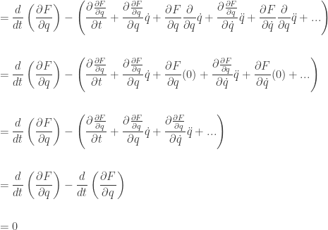
$\displaystyle{\begin{aligned} &\frac{\partial \dot F}{\partial \dot q} \\ \\ &= \frac{\partial }{\partial \dot q} \left( \frac{\partial F}{\partial t} + \frac{\partial F}{\partial q} \dot q + \frac{\partial F}{\partial \dot q} \ddot q + ... \right) \\ \\ &= \frac{\partial }{\partial \dot q} \frac{\partial F}{\partial t} + \left( \frac{\partial }{\partial \dot q}\frac{\partial F}{\partial q} \right) \dot q + \frac{\partial F}{\partial q} \frac{\partial }{\partial \dot q}\dot q + \left( \frac{\partial }{\partial \dot q}\frac{\partial F}{\partial \dot q} \right) \ddot q + \frac{\partial F}{\partial \dot q} \frac{\partial }{\partial \dot q}\ddot q + ... \\ \\ &= \frac{\partial }{\partial \dot q} \frac{\partial F}{\partial t} + \left( \frac{\partial }{\partial \dot q}\frac{\partial F}{\partial q} \right) \dot q + \frac{\partial F}{\partial q} (1) + \left( \frac{\partial }{\partial \dot q}\frac{\partial F}{\partial \dot q} \right) \ddot q + \frac{\partial F}{\partial \dot q} (0) + ... \\ \\ &= \frac{\partial }{\partial \dot q} \frac{\partial F}{\partial t} + \left( \frac{\partial }{\partial \dot q}\frac{\partial F}{\partial q} \right)\dot q + \frac{\partial F}{\partial q} + \left( \frac{\partial }{\partial \dot q}\frac{\partial F}{\partial \dot q}\right) \ddot q + ... \\ \\ &= \left[ \frac{\partial \frac{\partial }{\partial \dot q} F}{\partial t} + \left( \frac{\partial \frac{\partial }{\partial \dot q} F}{\partial q} \right)\dot q + \left( \frac{\partial \frac{\partial }{\partial \dot q} F}{\partial \dot q}\right) \ddot q + ... \right] + \frac{\partial F}{\partial q} \\ \\ &= \frac{d}{dt} \frac{\partial F }{\partial \dot q} + \frac{\partial F}{\partial q} \\ \\ \end{aligned}}$

If $\displaystyle{ L' = L + D_t F }$ depends on $\displaystyle{ \{t, q, Dq\} }$ only, then $\displaystyle{ F }$ will depend on $\displaystyle{ \{t, q\} }$ only.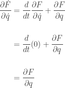

$\displaystyle{\begin{aligned} \frac{\partial \dot F}{\partial \dot q} &= \frac{d}{dt} \frac{\partial F }{\partial \dot q} + \frac{\partial F}{\partial q} \\ \\ &= \frac{d}{dt} (0) + \frac{\partial F}{\partial q} \\ \\ &= \frac{\partial F}{\partial q} \\ \\ \end{aligned}}$

[guess]

— Me@2022-06-03 09:04:37 PM

Ex 1.25 Properties of Dt, 3

Posted on May 24, 2022 by rpflee

Structure and Interpretation of Classical Mechanics

Demonstrate that …

d . $\displaystyle{D_t (H \circ G) = (DH \circ G) D_t G}$

~~~

$\displaystyle{ \begin{aligned} &D_t (HG) \circ \Gamma[q] (t) \\ \end{aligned} }$

$\displaystyle{ \begin{aligned} &= \partial_0 \left[ (H \circ G) (t, q, v, a, ...) \right] \\ &+ \partial_1 \left[ (H \circ G) (t, q, v, a, ...) \right] v(t) \\ &+ \partial_2 \left[ (H \circ G) (t, q, v, a, ...) \right] a(t) + ... \\ \end{aligned} }$

$\displaystyle{ \begin{aligned} &= \partial_0 \left[ H (G (t, q, v, a, ...)) \right] \\ &+ \partial_1 \left[ H (G (t, q, v, a, ...)) \right] v(t) \\ &+ \partial_2 \left[ H (G (t, q, v, a, ...)) \right] a(t) + ... \\ \end{aligned} }$

$\displaystyle{ \begin{aligned} &= D (H (G (t, q, v, a, ...))) \partial_0 G (t, q, v, a, ...) \\ &+ D (H (G (t, q, v, a, ...))) \partial_1 G (t, q, v, a, ...) v(t) \\ &+ D (H (G (t, q, v, a, ...))) \partial_2 G (t, q, v, a, ...) a(t) + ... \\ \end{aligned} }$

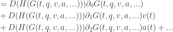
$\displaystyle{ \begin{aligned} &= D (H (G (t, q, v, a, ...))) \left[ \partial_0 G (t, q, ...) + \partial_1 G (t, q, ...) v(t) + \partial_2 G (t, q, ...) a(t) + ... \right] \\ \end{aligned} }$

$\displaystyle{ \begin{aligned} &= D ( (H \circ G) \circ \Gamma[q] (t) ) D_t G \circ \Gamma[q] (t) \\ \end{aligned} }$

$\displaystyle{ \begin{aligned} &= D_G (H \circ G) \circ \Gamma[q] (t) D_t G \circ \Gamma[q] (t) \\ \end{aligned} }$

$\displaystyle{ (fg) [q] \equiv f[q] g[q]}$

$\displaystyle{ \begin{aligned} &= \{ [D_G (H \circ G)] D_t G \} \circ \Gamma[q] (t) \\ \end{aligned} }$

— Me@2022-05-23 03:18:43 PM

Lisp macros 3

Posted on May 23, 2022 by rpflee

Power

Macros are one of the things that make Lisp so extensible, because they let you transform arbitrary code into other arbitrary code. This is true for macros in languages like C too, but Common Lisp macros are different because they’re part of the language.

In C you have a layer of macros on top, written in a preprocessor macro language. The macro layer and the language layer are separate from each other, with the macro layer providing one one extra level of abstractive power (which, don’t get me wrong, is certainly useful).

In Common Lisp, you write macros in Common Lisp itself. You can then use those macros to write functions, and use those functions to write more macros. Instead of two stratified layers it’s a feedback loop of abstractive power.

— A Road to Common Lisp

— Steve Losh

2022.05.22 Sunday ACHK

Watermelon

Posted on May 14, 2022 by rpflee

1990s, 19

(package-initialize)

(custom-set-variables
 '(cua-mode t nil (cua-base))
 '(custom-enabled-themes (quote (leuven))))
(custom-set-faces
 )

(set-register ?e '(file . "~/.emacs"))

(prefer-coding-system 'utf-8)

;;;;;;;;;;;;;;;;;;;;;;;;;;;;;;;;;;;;;;;;;;;;;;

(defun backup-dot-emacs ()
  (interactive)

  (save-buffer)

  (setq backup-path (format "%s%s%s" 
              "/path_to_the_backup_folder/ubuntu_dot_emacs_" 
              (format-time-string "%Y_%m_%d_%I_%M_%S_%p")  
              ".el"))
  
  (write-file backup-path 'confirm)

  (setq original-cursor (point))

  (kill-buffer) 
  (find-file "~/.emacs")

  (goto-char original-cursor)
)

(global-set-key (kbd "C-`") 'backup-dot-emacs)

;;;;;;;;;;;;;;;;;;;;;;;;;;;;;;;;;;;;;;;;;;;;;;


(set-register ?d '(file . "/path_to_the_blog_folder/dialogue59.txt"))

;;;;;;;;;;;;;;;;;;;;;;;;;;;;;;;;;;;;;;;;;;;;;;

(defun backup-blogging-tray ()
  (interactive)
  (save-buffer)

  (setq return-file-name (buffer-file-name))

  (setq backup-path (format "%s%s%s" 
                "/path_to_the_backup_folder/blogging_tray_" 
                (format-time-string "%Y_%m_%d_%I_%M_%S_%p")  
                ".txt"))

  (write-file backup-path 'confirm)

  (setq original-cursor (point))

  (kill-buffer) 

  (find-file return-file-name)

  (goto-char original-cursor)
 
)

(global-set-key (kbd "C-x C-a") 'backup-blogging-tray)

;;;;;;;;;;;;;;;;;;;;;;;;;;;;;;;;;;;;;;;;;;;;;;

— Me@2022.05.14 05:10:49 PM

Ex 1.25 Properties of Dt, 2

Posted on May 14, 2022 by rpflee

Structure and Interpretation of Classical Mechanics

Demonstrate that …

b. $\displaystyle{D_t (c F) = c D_t F}$

c. $\displaystyle{D_t (F G) = F D_t G + (D_t F) G}$

~~~

$\displaystyle{ \begin{aligned} &D_t (c F) \circ \Gamma[q] (t) \\ \end{aligned} }$

$\displaystyle{ \begin{aligned} &= \partial_0 \left[c F(t, q, v, a, ...) \right] + \partial_1 \left[c F(t, q, v, a, ...) \right] v(t) + \partial_2 \left[c F(t, q, v, a, ...) \right] a(t) + ... \end{aligned} }$

$\displaystyle{ \begin{aligned} &= c \partial_0 F(t, q, v, a, ...) + c \partial_1 F(t, q, v, a, ...) v(t) + c \partial_2 F(t, q, v, a, ...) a(t) + ... \end{aligned} }$

$\displaystyle{ \begin{aligned} &= c \left[ \partial_0 F(t, q, v, a, ...) + \partial_1 F(t, q, v, a, ...) v(t) + \partial_2 F(t, q, v, a, ...) a(t) + ... \right] \end{aligned} }$

$\displaystyle{ \begin{aligned} &= c D_t F \circ \Gamma[q] (t) \\ \end{aligned} }$

$\displaystyle{ \begin{aligned} &D_t (FG) \circ \Gamma[q] (t) \\ \end{aligned} }$

$\displaystyle{ \begin{aligned} &= \partial_0 \left[ F(t, q, v, a, ...) G(t, q, v, a, ...) \right] \\ &+ \partial_1 \left[ F(t, q, v, a, ...) G(t, q, v, a, ...) \right] v(t) \\ &+ \partial_2 \left[ F(t, q, v, a, ...) G(t, q, v, a, ...) \right] a(t) + ... \\ \end{aligned} }$

$\displaystyle{ \begin{aligned} &= \left[ \partial_0 F(t, q, v, a, ...) \right] G(t, q, v, a, ...) + F(t, q, v, a, ...) \partial_0 G(t, q, v, a, ...) \\ &+ \left\{ \left[ \partial_1 F(t, q, v, a, ...) \right] G(t, q, v, a, ...) + F(t, q, v, a, ...) \partial_1 G(t, q, v, a, ...) \right\} v(t) \\ &+ \left\{ \left[ \partial_2 F(t, q, v, a, ...) \right] G(t, q, v, a, ...) + F(t, q, v, a, ...) \partial_2 G(t, q, v, a, ...) \right\} a(t) + ... \\ \end{aligned} }$

$\displaystyle{ \begin{aligned} &= \left[ \partial_0 F(t, q, v, a, ...) \right] G(t, q, v, a, ...) \\ &+ \left[ \partial_1 F(t, q, v, a, ...) \right] G(t, q, v, a, ...) v(t) \\ &+ \left[ \partial_2 F(t, q, v, a, ...) \right] G(t, q, v, a, ...) a(t) + ... \\ \\ &+ F(t, q, v, a, ...) \partial_0 G(t, q, v, a, ...) \\ &+ F(t, q, v, a, ...) \partial_1 G(t, q, v, a, ...) v(t) \\ &+ F(t, q, v, a, ...) \partial_2 G(t, q, v, a, ...) a(t) + ... \\ \end{aligned} }$

$\displaystyle{ \begin{aligned} &= \left[ \partial_0 F(t, q, v, a, ...) + \partial_1 F(t, q, v, a, ...) v(t) + \partial_2 F(t, q, v, a, ...) a(t) + ... \right] G(t, q, v, a, ...) \\ &+ F(t, q, v, a, ...) \left[ \partial_0 G(t, q, v, a, ...) + \partial_1 G(t, q, v, a, ...) v(t) + \partial_2 G(t, q, v, a, ...) a(t) + ... \right] \\ \end{aligned} }$

$\displaystyle{ \begin{aligned} &= \left\{ D_t F \circ \Gamma[q] (t) \right\} G(t, q, v, a, ...) + F(t, q, v, a, ...) D_t G \circ \Gamma[q] (t) \\ \end{aligned} }$

$\displaystyle{ \begin{aligned} &= \left\{ D_t F \circ \Gamma[q] (t) \right\} G \circ \Gamma[q] (t) + F \circ \Gamma[q] (t) D_t G \circ \Gamma[q] (t) \\ \end{aligned} }$

The meaning of $\displaystyle{\delta_\eta (fg)[q]}$ is

$\displaystyle{\delta_\eta (f[q]g[q])}$

$\displaystyle{ \begin{aligned} &D_t (FG) \circ \Gamma[q] (t) \\ \end{aligned} }$

$\displaystyle{ \begin{aligned} &= \left\{ D_t F \circ \Gamma[q] (t) \right\} G \circ \Gamma[q] (t) + F \circ \Gamma[q] (t) D_t G \circ \Gamma[q] (t) \\ \end{aligned} }$

$\displaystyle{ \begin{aligned} &= \left[ (D_t F) G + F D_t G \right] \circ \Gamma[q] (t) \\ \end{aligned} }$

$\displaystyle{ \begin{aligned} D_t (FG) \circ \Gamma[q] (t) &= \left[ (D_t F) G + F D_t G \right] \circ \Gamma[q] (t) \\ \\ D_t (FG) &= (D_t F) G + F D_t G \\ \end{aligned} }$

— Me@2022.05.12 07:02:30 PM

Junkions

Posted on May 7, 2022 by rpflee

output = system.exec_command("date +%Y.%m.%d")
output += " "
output += system.exec_command("date +%I:%M:%S")
output += " "
output += system.exec_command("date +%p")

clipboard.fill_clipboard(output.upper())
keyboard.send_keys("<ctrl>+v")

output = system.exec_command("date +%Y.%m.%d")
output += " "
output += system.exec_command("date +%A")
output += " (c) All rights reserved by "

clipboard.fill_clipboard(output)
keyboard.send_keys("<ctrl>+v")

output = system.exec_command("date +_%Y_%m_%d_")
output += system.exec_command("date +_%H_%M_%S_%p")

clipboard.fill_clipboard(output.upper())
keyboard.send_keys("<ctrl>+v")

— Me@2022.05.07 11:27:28 AM

The Lisp debugger

Posted on May 5, 2022 by rpflee

oo101 7 days ago [-]

There are a few ways in which the shared objects method you suggest does not match the full power of Lisp debugging.

First of all, when a C program crashes, it just crashes. There is no REPL. There is only a core dump. So any live-debugging you plan to do is after the fact. After you have seen a crash, you would now begin to prepare for the next crash by launching your process via GDB or restarting your process and attaching a GDB to it. Whether a similar crash would occur again or not or when it would occur again depends on the nature of the bug. Now contrast this with Lisp debugging when your program crashes, it stops there and offers you an REPL to interact with the program right then. There is no need to wait for the next crash.

Secondly, when you debug with GDB, you would be dealing with syntaxes: The syntax of C that we are so familiar with. The GDB syntax to investigate the problem that we may be less familiar with. When the Lisp debugger offers the REPL to you, you are working with Lisp again. Your compiler, debugger, program, etc. all are part of the same unified environment where you just execute Lisp code to debug your issue.

Finally, putting your code in shared objects and reloading them requires you to go through the complete write-build-test-debug cycle. And then what do you do if your shared object itself crashes? With Lisp you skip the write-build-test part when all you want to do is debug an error. You jump straight to the debug part of the cycle and begin investigating the runtime state. And it works the same in a uniform manner whether your main program crashes or a dependency crashes.

— A Road to Common Lisp

— Hacker News

2022.05.05 Thursday ACHK

AutoKey

Posted on April 28, 2022 by rpflee

First photo, 3 | 1990, 3


output = system.exec_command("date +%Y.%m.%d")
keyboard.send_keys(output + " ")
output = system.exec_command("date +%I:%M")
keyboard.send_keys(output + " ")
output = system.exec_command("date +%p")
keyboard.send_keys(output)


output = system.exec_command("date +%Y.%m.%d")
keyboard.send_keys(output + " ")
output = system.exec_command("date +%A")
keyboard.send_keys(output)
output = " (c) All rights reserved by "
keyboard.send_keys(output)


output = system.exec_command("date +_%Y_%m_%d_")
keyboard.send_keys(output)
output = system.exec_command("date +_%H_%M_%S_%p")
keyboard.send_keys(output)

— Me@2022.04.28 09:04 AM

Physics Town

continues

Category Archives: software

SICMUtils

Common Lisp Reloaded

Cyclic coordinate

Functional programming jargon in plain English

Matrix calculus

Common Lisp vs Racket

1.7 Evolution of Dynamical State, 2.2

1.7 Evolution of Dynamical State, 2.1

1.7 Evolution of Dynamical State

C-h ?

Ex 1.27 Identifying total time derivatives

3Blue1Brown

Ex 1.26 Lagrange equations for total time derivatives

Ex 1.25 Properties of Dt, 3

Lisp macros 3

Watermelon

Ex 1.25 Properties of Dt, 2

Junkions

The Lisp debugger

AutoKey