Circus

Posted on April 7, 2022 by rpflee

drblast on Oct 27, 2010 | next [–]

Living with one child is like living with a demanding, but mostly reasonable, roommate who really likes spending time with you until she goes to bed early.

Having two or more children is like living in a circus where all the performers are deaf.

— Ask HN: How does having a baby change your life?

2022.04.07 Thursday ACHK

伏線驅動程式 1.3

Posted on April 6, 2022 by rpflee

這段改編自 2010 年 10 月 14 日的對話。

為何我在幾年前，會在這裡教書呢？

因為之前我找到工作的那間補習社，言而無信。我應徵面試完時，面試職員說會聘請我，叫我等消息。一段時間後，還未有消息。

一般而言，面試職員只會，叫人「等消息」。想聘請的話，自然會聯絡我。沒有消息的話，就代表不聘用。所以，在通常的情況下，沒有消息時，並不需要再，打電話去詢問。

但是，那次的面試職員是說「會聘請」，稍後再聯絡。所以，長久沒有消息時，我致電詢問。但是，接線人員的答覆是，會再聯絡；即是模稄兩可。隔了數天之後，我又再問多一次，究竟是聘不聘用。

「我可不可以與，當天的面試人員，傾一傾談？」

「不可以。」

仍然沒有答覆。

答覆我一句，聘請還是不聘請，並不是問題。最滋擾人的是，不置可否。

「究竟那間補習社會聘請我，我應該等待那份工作，還是立刻找其他呢？」

當然，當年還年輕，才會犯這類低級錯誤。

愛情上，找到男／女朋友前，要不斷結識新的朋友，尤其異性。

事業上，莫講話我當時，未有固定工作，即使正職在職，亦即是話，任何情況下，本應不斷去面試，尋找新機遇。那樣，才可以為我的未來太太和子女，提供到基本生活的經濟保障。

記住，你可以對，你的金錢和工作有感情，但千萬不要對，你的公司和職位有感情。我年青就，就是犯了「對公司和職位有感情」這重大錯失，導致自己和家人，受了一些不必要之苦；亦導致自己可能不會有，未來的家人。

— Me@2022-03-08 12:06:18 PM

1990s, 18

Posted on April 6, 2022 by rpflee

— Me@2022-04-06 10:02:58 AM

Ex 1.24 Constraint forces, 1.2

Posted on April 5, 2022 by rpflee

Ex 1.22 Driven pendulum, 3.2

Structure and Interpretation of Classical Mechanics

Find the tension in an undriven planar pendulum.

~~~

[guess]


(define ((q->r x_s y_s l) local)
  (let* ((q (coordinate local))
         (t (time local))
         (theta (ref q 0))
         (c (ref q 1))
         (F (ref q 2)))
    (up (+ (x_s t) (* c (sin theta)))
        (- (y_s t) (* c (cos theta)))
        F)))

(let* ((xs (literal-function 'x_s))
       (ys (literal-function 'y_s))
       (q (up (literal-function 'theta)
              (literal-function 'c)
              (literal-function 'F))))
  (show-expression ((compose (q->r xs ys 'l) (Gamma q)) 't)))


(define (L-theta m l x_s y_s U)
  (compose
   (L-driven-free m l x_s y_s U) (F->C (q->r x_s y_s l))))

(let* ((U (U-gravity 'g 'm))
       (xs (literal-function 'x_s))
       (ys (literal-function 'y_s))
       (q (up (literal-function 'theta)
              (literal-function 'c)             
              (literal-function 'F)))
       (L (L-theta 'm 'l xs ys U)))
  (show-expression (L ((Gamma q) 't))))

(/
 (+ (* l m ((D x_s) t) (c t) ((D theta) t) (cos (theta t)))
    (* 1/2 l m (expt (c t) 2) (expt ((D theta) t) 2))
    (* l m (c t) ((D theta) t) (sin (theta t)) ((D y_s) t))
    (* g l m (c t) (cos (theta t)))
    (* l m ((D x_s) t) ((D c) t) (sin (theta t)))
    (* -1 l m ((D c) t) (cos (theta t)) ((D y_s) t))
    (* -1 g l m (y_s t))
    (* 1/2 l m (expt ((D x_s) t) 2))
    (* 1/2 l m (expt ((D c) t) 2))
    (* 1/2 l m (expt ((D y_s) t) 2))
    (* 1/2 (expt l 2) (F t))
    (* -1/2 (expt (c t) 2) (F t)))
 l)


(let* ((U (U-gravity 'g 'm))
       (xs (literal-function 'x_s))
       (ys (literal-function 'y_s))
       (q (up (literal-function 'theta)
              (literal-function 'c)
              (literal-function 'F)))
       (L (L-theta 'm 'l xs ys U)))
  (show-expression (((Lagrange-equations L) q) 't)))


(let* ((U (U-gravity 'g 'm))
       (xs (lambda (t) 0))
       (ys (lambda (t) 'l))
       (q (up (literal-function 'theta)
              (lambda (t) 'l)
              (literal-function 'F)))
       (L (L-theta 'm 'l xs ys U)))
  (show-expression (((Lagrange-equations L) q) 't)))

$\displaystyle{F(t) = l m \left[D \theta(t)\right]^2 + g m \cos \theta(t)}$

[guess]

— Me@2022-04-05 04:16:51 PM

Dynamical pictures

Posted on April 5, 2022 by rpflee

Comparison of pictures

The Heisenberg picture is closest to classical Hamiltonian mechanics (for example, the commutators appearing in the above equations directly correspond to classical Poisson brackets). The Schrödinger picture, the preferred formulation in introductory texts, is easy to visualize in terms of Hilbert space rotations of state vectors, although it lacks natural generalization to Lorentz invariant systems. The Dirac picture is most useful in nonstationary and covariant perturbation theory, so it is suited to quantum field theory and many-body physics.

Summary comparison of evolutions

— Wikipedia on Dynamical pictures

2022.04.05 Tuesday ACHK

地獄篇 9

Posted on April 4, 2022 by rpflee

外在世界是地獄，心中宇宙是天堂；把知識和想像化成現實，就是把地獄天堂化。

— Me@2011.10.05

兩見終情

Posted on April 3, 2022 by rpflee

這段改編自 2021 年 12 月 9 日的對話。

如果你將來遇到，一個你心儀對象的話，千萬不要以為，她一定是你未來太太。亦即是話，即使是「一見鍾情」，那也只是感覺，未必反映實情；「兩見如何」還要相處過才知道。

幾十年前，我曾經遇到，一位心儀的女士。我與她有著，電影《情留半天》級數的對話。她也對我有意思。我怎麼知道呢？

當時我煩惱著，她會否已有男朋友。但是，我又不好意思問。反而，她有天突然問我，有沒有女朋友。

如果可以定期見面，我們理應可以，自然發展成情侶。

不幸，她有著關鍵的缺點，而我又改變不到。例如，她會連續五次失約。

— Me@2022-04-02 04:39:11 PM

Stay Hungry, Stay Foolish

Posted on April 1, 2022 by rpflee

求知若飢虛懷若愚

— Steve Jobs

Quick Calculation 3.1

Posted on April 1, 2022 by rpflee

A First Course in String Theory

Verify that $\displaystyle{\vec E}$ , as given in (3.8), is invariant under the gauge transformation (3.10).

~~~

Eq. (3.8):

$\displaystyle{\vec E = - \frac{1}{c} \frac{\partial \vec A}{\partial t} - \nabla \Phi}$

Eq. (3.10):

$\displaystyle{ \begin{aligned} \Phi' &= \Phi - \frac{1}{c} \frac{\partial \epsilon}{\partial t} \\ \vec A' &= \vec A + \nabla \epsilon \\ \end{aligned} }$

$\displaystyle{ \begin{aligned} \vec E' &= - \frac{1}{c} \frac{\partial \vec A'}{\partial t} - \nabla \Phi' \\ &= - \frac{1}{c} \frac{\partial \vec A}{\partial t} - \frac{1}{c} \frac{\partial}{\partial t} \left( \nabla \epsilon \right) - \nabla \Phi + \frac{1}{c} \nabla \frac{\partial \epsilon}{\partial t} \\ &= \vec E \\ \end{aligned} }$

— Me@2022-04-01 03:34:28 PM

Huygens’ principle, 1.1

Posted on March 30, 2022 by rpflee

Why are there no backward secondary wavefronts?

A secondary wave source is of different nature from a primary wave source. Consider an one dimensional transverse wave on a string:

Primary wave source is activated by the force from above, and then the wave propagates to both directions. Secondary wave source is activated by the particle on the left.

Primary wave source energy is from outside the string. Secondary wave source energy is from an adjacent string molecule.

When the secondary source S reaches its maximum, although it drags both P and Q, they are in different situations. At that moment, while the instantaneous velocity of Q is upward, that of P is downward.

Note that the red arrow at P is the force on P by S. It is not the net force on P.

— Me@2022-03-09 11:14:07 PM

惜此際 5

Posted on March 29, 2022 by rpflee

先唔講地唔地獄，但係因為有呢種人生觀，就算瓜咗，呢種思想模式都只會帶佢到呢啲境界嘅地方，到咗嗰度，如果佢都係咁睇野，結局又係揀自殺，咁樣不斷自殺，經歷一次又一次咁嘅局面，咁嘅經歷真係唔知算唔算地獄，可能佢都唔知經歷過幾多次呢款生生死死了，只有佢自己救到自己，其實心態改變一下就ok了，無野帶到黎，亦無野帶得走，咁認真做乜呢

—

2022.03.29 Tuesday ACHK

伏線驅動程式 1.2

Posted on March 29, 2022 by rpflee

這段改編自 2010 年 10 月 14 日的對話。

時間的結構是這樣的，未來片面不全知，成果可預不可期。

我發覺人生，即使愛情以外的範疇，主要的演變都是，身不由己式，依靠伏線來驅動。例如，此時此境此地，我是來教你們物理，順便講道理。

我又是如何認識你們的呢？

因為 HYC 問我有沒有時間，教他們「數學與統計」科；她順便問我，有沒有時間去，教其他同學物理科。

為何 HYC 會問我數學呢？

因為之前臨近中五會考，我在教你們中五師妹 CKY 的「附加數學」時，HYC 見到我。

為何 CKY 會找我教「附加數學」呢？

因為再之前，我在教你一位，中七師姐 CPM 物理時，CKY 見到我。

為何我會教 CPM 物理呢？

因為我在這裡教書時，她是我的數學科學生。臨近中七高考時，我問她有沒有物理問題要問我。

為何我在幾年前，會在這裡教書呢？

因為之前我找到工作的那間補習社，言而無信。我應徵面試完時，面試職員說會聘請我，叫我等消息。一段時間後，還未有消息。

— Me@2022-03-08 12:06:18 PM

Politician

Posted on March 27, 2022 by rpflee

— Me@2022-03-26 07:51:29 PM

2022.03.26 Saturday ACHK

Ex 1.22 Driven pendulum, 3.1

Posted on March 26, 2022 by rpflee

Ex 1.24 Constraint forces, 1.1

Structure and Interpretation of Classical Mechanics

~~~

[guess]

$\displaystyle{ \begin{aligned} m \ddot{y} &= F \cos \theta - mg \\ m \ddot{x} &= - F \sin \theta \\ \end{aligned}}$

$\displaystyle{ \begin{aligned} m \ddot{y} &= F \frac{y_s - y}{l} - mg \\ m \ddot{x} &= - F \frac{x - x_s}{l} \\ \sqrt{(x_s - x)^2 + (y_s - y)^2} &= l \\ \end{aligned}}$

$\displaystyle{ \begin{aligned} y_s &= l \\ x_s &= 0 \\ \end{aligned}}$

$\displaystyle{ \begin{aligned} m \ddot{y} &= F \frac{l - y}{l} - mg \\ m \ddot{x} &= - F \frac{x}{l} \\ \sqrt{x^2 + (l - y)^2} &= l \\ \end{aligned}}$


(define (KE-particle m v)
  (* 1/2 m (square v)))
 
(define ((extract-particle pieces) local i)
  (let* ((indices (apply up (iota pieces (* i pieces))))
         (extract (lambda (tuple)
                    (vector-map (lambda (i)
                                  (ref tuple i))
                                indices))))
    (up (time local)
        (extract (coordinate local))
        (extract (velocity local)))))
 
(define (U-constraint q0 q1 F l)
  (* (/ F (* 2 l))
     (- (square (- q1 q0))
        (square l))))
 
(define ((U-gravity g m) q)
  (let* ((y (ref q 1)))
    (* m g y))) 

(define ((L-driven-free m l x_s y_s U) local)
  (let* ((extract (extract-particle 2))
      
     (p (extract local 0))
     (q (coordinate p))
     (qdot (velocity p))
      
     (F (ref (coordinate local) 2)))
   
    (- (KE-particle m qdot)
       (U q)
       (U-constraint (up (x_s (time local)) (y_s (time local)))
             q
             F
             l))))

(let* ((U (U-gravity 'g 'm))
       (x_s (literal-function 'x_s))
       (y_s (literal-function 'y_s))
       (L (L-driven-free 'm 'l x_s y_s U))
       (q-rect (up (literal-function 'x)
                   (literal-function 'y)
                   (literal-function 'F))))
  (show-expression
   ((compose L (Gamma q-rect)) 't)))

$\displaystyle{ L = \frac{1}{2} m \left[(Dx)^2 + (Dy)^2 \right] - mgy - \frac{F}{2l} \left[ (x-x_s)^2 + (y-y_s)^2 - l^2 \right] }$


(let* ((U (U-gravity 'g 'm))
       (x_s (literal-function 'x_s))
       (y_s (literal-function 'y_s))
       (L (L-driven-free 'm 'l x_s y_s U))
       (q-rect (up (literal-function 'x)
                   (literal-function 'y)
                   (literal-function 'F))))
  (show-expression
   (((Lagrange-equations L) q-rect) 't)))

$\displaystyle{ \begin{aligned} mD^2x(t) + \frac{F(t)}{l} \left[x(t) - x_s(t)\right] &= 0 \\ mg + m D^2y(t) + \frac{F(t)}{l} [y(t) - y_s(t)] &= 0 \\ -l^2 + [y(t)-y_s(t)]^2 + [x(t)-x_s(t)]^2 &= 0 \\ \end{aligned}}$


(define ((F->C F) local)
  (->local (time local)
           (F local)
           (+ (((partial 0) F) local)
              (* (((partial 1) F) local) 
                 (velocity local)))))

(define ((q->r x_s y_s l) local)
  (let* ((q (coordinate local))
         (t (time local))
         (theta (ref q 0))
         (F (ref q 1)))
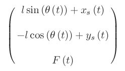
    (up (+ (x_s t) (* l (sin theta)))
        (- (y_s t) (* l (cos theta)))
        F)))

(let ((q (up (literal-function 'theta)             
             (literal-function 'F))))
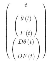
  (show-expression (q 't)))


(let* ((x_s (literal-function 'x_s))
       (y_s (literal-function 'y_s))
       (q (up (literal-function 'theta)             
              (literal-function 'F))))
  (show-expression ((Gamma q) 't)))


(let* ((xs (literal-function 'x_s))
       (ys (literal-function 'y_s))
       (q (up (literal-function 'theta)             
              (literal-function 'F))))
  (show-expression ((compose (q->r xs ys 'l) (Gamma q)) 't)))


(let* ((xs (literal-function 'x_s))
       (ys (literal-function 'y_s))
       (q (up (literal-function 'theta)             
              (literal-function 'F))))
  (show-expression ((F->C (q->r xs ys 'l)) ((Gamma q) 't))))



(define (L-theta m l x_s y_s U)
  (compose
   (L-driven-free m l x_s y_s U) (F->C (q->r x_s y_s l))))

(let* ((U (U-gravity 'g 'm))
       (xs (literal-function 'x_s))
       (ys (literal-function 'y_s))
       (q (up (literal-function 'theta)             
              (literal-function 'F))))
  (show-expression ((Gamma
                    (compose (q->r xs ys 'l) (Gamma q)))
                    't)))



(let* ((U (U-gravity 'g 'm))
       (xs (literal-function 'x_s))
       (ys (literal-function 'y_s))
       (q (up (literal-function 'theta)             
              (literal-function 'F))))
  (show-expression (U ((compose (q->r xs ys 'l) (Gamma q)) 't))))


(let* ((U (U-gravity 'g 'm))
       (xs (literal-function 'x_s))
       (ys (literal-function 'y_s))
       (q (up (literal-function 'theta)             
              (literal-function 'F))))
  (show-expression ((L-driven-free 'm 'l xs ys U)
		    ((Gamma (compose (q->r xs ys 'l) (Gamma q))) 't))))



(let* ((U (U-gravity 'g 'm))
       (xs (literal-function 'x_s))
       (ys (literal-function 'y_s))
       (q (up (literal-function 'theta)             
              (literal-function 'F))))
  (show-expression ((L-theta 'm 'l xs ys U) ((Gamma q) 't))))

$\displaystyle{ \begin{aligned} L_\theta &= \frac{1}{2} m (D x_s(t))^2 + \frac{1}{2} m (D y_s(t))^2 - m g \left[ y_s(t) - l \cos \theta(t) \right] \\ &+ \frac{1}{2} m l^2 (D \theta(t))^2 + lm D \theta(t) \left[ D x_s(t) \cos \theta(t) + \sin \theta(t) D y_s(t) \right] \\ \end{aligned}}$

[guess]

— Me@2022-03-24 04:38:10 PM

EPR paradox, 12.2

Posted on March 24, 2022 by rpflee

…

Experiment C:

What if during Experiment A, the observer changes his mind to turn on the detector before the particle’s arrival?

Explanation X:

We should regard this whole process as an experiment-setup.

The probability patterns encoded in the quantum state is of this experiment-setup, which in this case is equivalent to Experiment B. With respect to this experiment-process/experiment-setup, the variable-to-be-measured is always in a mixed state.

The word “always” here means that a quantum state is not a physical state of a particle in physical spacetime during the experiment. Instead, it is a property (of a physical variable) of the experiment-setup (physical system) itself.

“Physical system” means the experimental-setup design, which includes not just objects and devices, but also operations.

However, for an experiment like Experiment C, doesn't the violation of Bell's inequality have proved that the spin of the particle is still in a superposition before the activation of the detector?

Let’s translate this question to a double-slit experiment version. (The consistency of the left detector and the right detector is as strange as the EPR consistency.)

Experiment C:

What if in the double-slit experiment, the detector is off when the particle is emitted, but the observer changes his mind to turn on the detector before the particle’s passing through of the double-slit plate?

Is the particle in a superposition or not when the detector is still off?

Instead of a superposition pure state, we should regard the particle path state as a mixed state, even before the detector is activated.

The reason is given in Explanation X.

However, for an experiment like Experiment C, doesn't the violation of Bell's inequality have proved that the path of the particle is still in a superposition before the activation of the detector?

The violation of Bell’s inequality should be interpreted in this way:

Experiment A:

If there is no detector activated throughout the experiment until the particle reaches the final screen, the resulting statistical pattern (aka the interference pattern) is possible only if the particle has no definite path. “An unknown but definite path exists” would not be able to create such statistics.

.

Experiment B:

If there is a detector activated since the beginning of the experiment, the particle path is in a mixed state since that beginning, meaning that the path is definite although unknown before measurement.

.

Experiment C:

What if in the double-slit experiment, the detector is off when the particle is emitted, but the observer changes his mind to turn on the detector before the particle’s passing through of the double-slit plate?

Is the particle in a superposition or not when the detector is still off?

After the detector is activated, the path is in a mixed state.

Before the detector is activated, regarding the path state as in a superposition or as in a mixed state makes no physical difference, because by definition, there is no measurement before the detector is activated.

Also, a superposition’s coefficients are always about the potential-activation of detectors.

A superposition state has a corresponding mixed state. The superposition coefficients can be modulus-squared to give the mixed state coefficients. That is the exact original meaning of the superposition coefficients. (This is the statistical interpretation given by Born rule.)

In other words, each coefficient in a superposition state by default encodes the probability of each potential measurement result.

However, in Experiment C, regarding the state as a superposition state before the activation of detector creates conceptual paradoxes, such as:

If the particle path variable has no definite state before measurement, how come the left detector and right detector always give consistent results?

This is the double-slit experiment version of the EPR paradox.

When the experimenter follows the plan of Experiment A, the particle path variable is always in a superposition, since the beginning of the experiment.

However, when he changes his mind to turn on the detector before the particle’s passing through of the double-slit plate, the particle path variable is always in a mixed state, since the beginning of the experiment.

Wouldn’t that create retro-causality?

It seems to be retro-causality, but it is not, because this description is a language shortcut only. The apparent violation of causality does not exist in the language longcut version, which is provided in Explanation X.

Also, due to the indistinguishability of identical particles, particle identities and thus particle trajectories are post hoc stories only.

In short, the violation of Bell’s inequality means that:

If there is no path detector activated throughout the experiment until the particle reaches the final screen, the path variable never has a definite value, known or unknown, throughout that experiment.

The violation of Bell’s inequality should not be applied to Experiment C, because it is not the case of “having no detector throughout the experiment”.

Also, note that we do not need the violation of Bell’s inequality to prove that the path variable has no definite state, known or unknown.

Just the interference pattern’s existence is already enough for us to do so.

— Me@2022-03-08 11:56:00 PM

What is a leader?

Posted on March 21, 2022 by rpflee

Someone who causes people to do that which they ought to do but which they would not do in his absence.

— John T. Reed

2022.03.21 Monday ACHK

十萬七千里 3

Posted on March 20, 2022 by rpflee

數學教育 7.3

這段改編自 2010 年 4 月 24 日的對話。

（安：另外，他提的另一個，有關學習數學的要點是，即使假設你在大學中，學到的數學，在日常生活中沒有用，單單是為獲取，那些嶄新的元素概念本身，就已經能夠令你有超能力；令你有一些，常人沒有的思考工具、比喻語言。）

…

再例如，在微積分之初，我們學到了「極限」這概念。有時一些數式，永遠不會達到某個數値，但是卻可以，無限迫近。

例如， $\displaystyle{\forall x,~~\frac{1}{x} \ne 0}$ ；意思是，無論你把 $\displaystyle{x}$ 設成任何數値， $\displaystyle{\frac{1}{x}}$ 都不會等於零。但是，你卻可以要求 $\displaystyle{\frac{1}{x}}$ ，任意接近零。

$\displaystyle{\lim_{x \to \infty} \frac{1}{x} = 0}$

例如，如果想 $\displaystyle{\frac{1}{x}}$ 與 $\displaystyle{0}$ 相差，少於 $\displaystyle{0.01}$ 的話，你就設 $\displaystyle{x = 101}$ ；如果想相差，少於 $\displaystyle{0.0001}$ 的話，你就設 $\displaystyle{x = 10001}$ ；如此類推。

這個原理用作，人生哲學的比喻的話，就是指，即使「目標不可能」，也不代表「要完全放棄」。亦即是話，即使你的一些人生目標，不可能實現，那也不代表你，完全沒有東西可以做。那「不可能的目標」或許可以，轉化為一個「可能的近似版本」。

例如，你的目標是「不勞而獲」，不用工作就有金錢收入。一般情形下，那是不可能。但是，「不勞而獲」有近似的版本嗎？

有，有一些。例如，「小勞大獲」可以嗎？又例如，找你喜歡的工作可以嗎？

快樂工作的話，工作就不再是「工作」了。你被迫做一件事的話，那件事就是「工作」。你即使沒有需要，也會因為喜好，而做一件事的話，那件事就是「娛樂」。

— Me@2022-03-14 05:11:29 PM

Game Boy

Posted on March 12, 2022 by rpflee

1990s, 17

2.11 Extra dimension and statistical mechanics, 3

Posted on March 10, 2022 by rpflee

A First Course in String Theory

(b) Assume that $\displaystyle{R \ll a}$ in such a way that …

…

~~~

[guess]

$\displaystyle{\frac{\hbar^2}{ma^2} \ll k T \ll \frac{\hbar^2}{mR^2}}$

$\displaystyle{ \begin{aligned} Z &= Z(a) \tilde{Z}(R) \\ \end{aligned}}$

$\displaystyle{ \begin{aligned} Z(a) &= \sum_{k=1}^\infty \exp\left[- \beta \left( \frac{\hbar^2}{2m} \right) \left(\frac{k \pi}{a} \right)^2 \right] \\ \tilde Z (R) &= 1 + 2 Z(R \pi) \\ \end{aligned}}$

$\displaystyle{\beta = \frac{1}{kT} \ll \frac{ma^2}{\hbar^2}}$

$\displaystyle{ \begin{aligned} Z(a) &\approx \frac{1}{\beta} \int_{x = 0}^\infty e^{\left[- \frac{1}{\beta} \left( \frac{\hbar^2}{2m} \right) \left(\frac{x \pi}{a} \right)^2 \right]} dx = \sqrt{\frac{m a^2}{2 \beta \pi \hbar^2}} \\ \end{aligned}}$

$\displaystyle{\beta \gg \frac{mR^2}{\hbar^2}}$

$\displaystyle{ \begin{aligned} Z(R\pi) &= \sum_{k=1}^\infty \exp\left[- \beta \left( \frac{\hbar^2}{2m} \right) \left(\frac{k}{R} \right)^2 \right] \\ &= \exp\left[- \beta \left( \frac{\hbar^2}{2mR^2} \right) \right] + ... \\ &= 1 - \beta \left( \frac{\hbar^2}{2mR^2} \right) + ... \\ \end{aligned}}$

$\displaystyle{ \begin{aligned} \tilde Z (R) &= 1 + 2 Z(R \pi) \\ &= 1 + 2 \sum_{k=1}^\infty \exp\left[- \beta \left( \frac{\hbar^2}{2m} \right) \left(\frac{k}{R} \right)^2 \right]\\ &= 1 + 2 \left\{ \exp\left[- \beta \left( \frac{\hbar^2}{2mR^2} \right) \right] + ... \right\} \\ \end{aligned}}$

[guess]

— Me@2022-03-10 10:56:10 AM

EPR paradox, 12.1

Posted on March 9, 2022 by rpflee

A wave function (for a particular variable) is an intrinsic property of a physical system.

“Physical system” means the experimental-setup design, which includes not just objects and devices, but also operations.

In other words, “where and when an observer should do what during the experiment” is actually part of your experimental-setup design, defining what probability distribution (for any particular variable) you (the observer) will get.

If the experimenter does not follow the original experiment design, such as not turning on the detector at the pre-defined time, then he is actually doing another experiment, which will have a completely different probability distribution (for any particular variable).

— Me@2022-02-18 07:40:14 AM

— Me@2022-02-22 07:01:40 PM

Note that different observers see different “physical systems”. They see different quantum states, because a quantum state is actually not a “state”, but a (statistical) property of a system, encoded in the superposition coefficients.

Experiment A:

In an EPR experiment, if it is by design that an observer will not turn on the detector, then the story should be that this experiment-setup is always in a superposition state (with respect to the variable-not-to-be-measured).

.

Experiment B:

In an EPR experiment, if it is by design that an observer will turn on the detector before a particle’s arrival, then the story should be that this experiment-setup is always in a mixed state (with respect to the variable-to-be-measured).

.

No concept of “wave function collapse” is needed.

What if during Experiment A, the observer changes his mind to turn on the detector before the particle's arrival?

He has actually replaced experiment-setup A with experiment-setup B.

Then is the experiment always in a superposition state? Or always in a mixed state?

As a language shortcut, you can say that the superposition wave function collapses at the moment of system replacement.

However, it is a language shortcut, a story only.

A story is not reality.

A story is post hoc.

physical definition

~ define unobservable events in terms of observable events

Any story would be fine as long as it is compatible with reality, aka measurement results.

But some stories are better than others.

Here, only the longcut version can avoid common meaningless questions.

Experiment C:

What if during Experiment A, the observer changes his mind to turn on the detector before the particle’s arrival?

We should regard this whole process as an experiment-setup.

The probability patterns encoded in the quantum state is of this experiment-setup, which in this case is equivalent to Experiment B. With respect to this experiment-process/experiment-setup, the variable-to-be-measured is always in a mixed state.

The word “always” here means that a quantum state is not a physical state of a particle in physical spacetime during the experiment. Instead, it is a property (of a physical variable) of the experiment-setup (physical system) itself.

“Physical system” means the experimental-setup design, which includes not just objects and devices, but also operations.

However, for an experiment like Experiment C, doesn't the violation of Bell's inequality have proved that the spin of the particle is still in a superposition before the activation of the detector?

Let’s translate this question to a double-slit experiment version.

…

— Me@2022-03-08 11:56:00 PM

Physics Town

continues

Circus

伏線驅動程式 1.3

1990s, 18

Ex 1.24 Constraint forces, 1.2

Dynamical pictures

地獄篇 9

兩見終情

Stay Hungry, Stay Foolish

Quick Calculation 3.1

Huygens’ principle, 1.1

惜此際 5

伏線驅動程式 1.2

Politician

Ex 1.22 Driven pendulum, 3.1

EPR paradox, 12.2

What is a leader?

十萬七千里 3

Game Boy

2.11 Extra dimension and statistical mechanics, 3

EPR paradox, 12.1